Tag Archives: 2D

The Beauty of Roots

For a nice introduction to roots and their fractal nature, see this post from 2011 on John Baez’s Azimuth blog or his 2023 UCR page here. Some of my code here is sourced from a great repository of interesting math visualizations from many others including the author of the pywonderland GitHub of Zhao Liang.

The SVG images below can be clicked to zoom in on another tab, but here is a Mathematica Notebook with Tooltip info on the selected roots. That SVG is 8000×8000, so you may have to <cntrl>- to zoom out to see any of the interesting parts (depending on your screen resolution and browser setup).
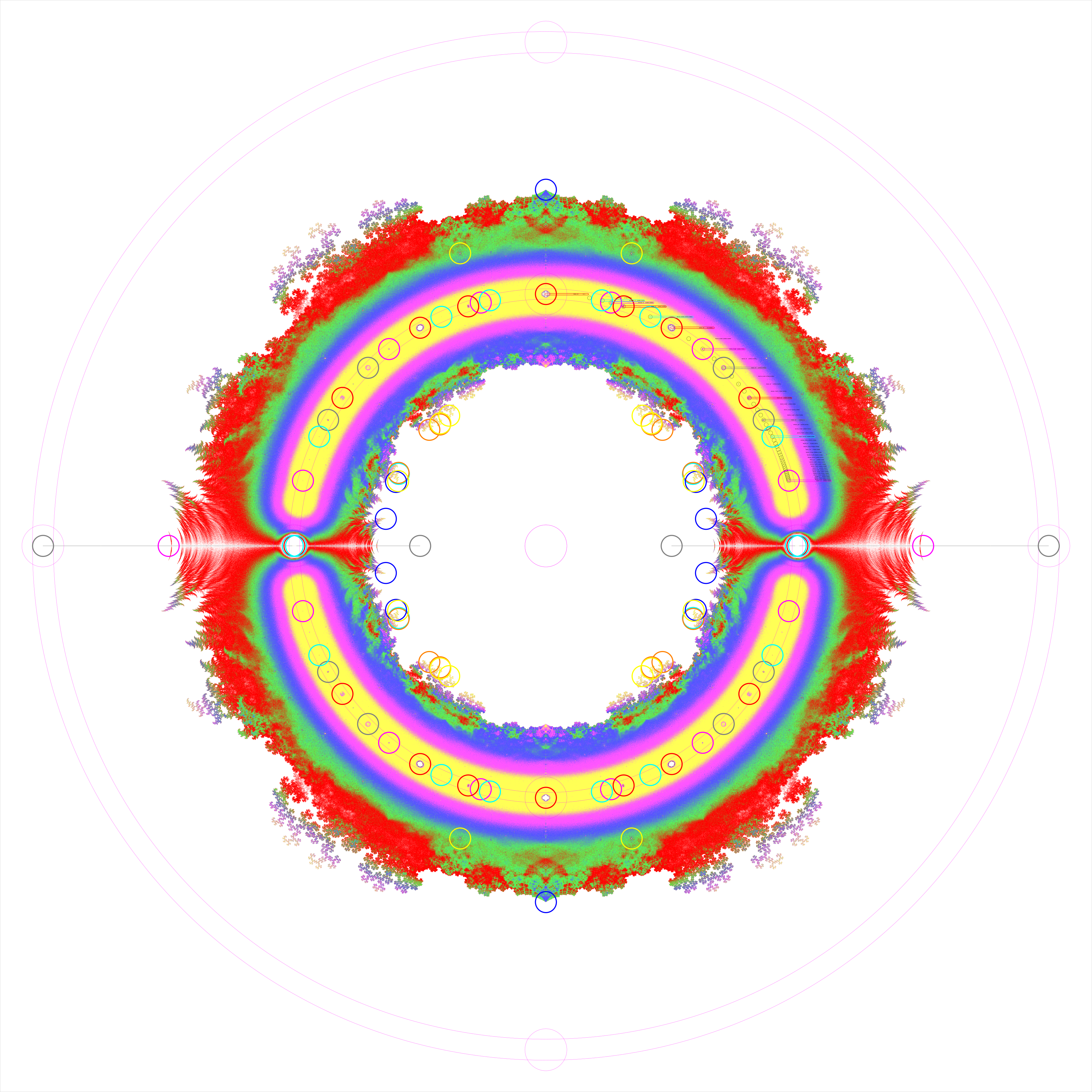
All roots of polynomials up to 224 (~16.7 million) with +/-1 coefficients.

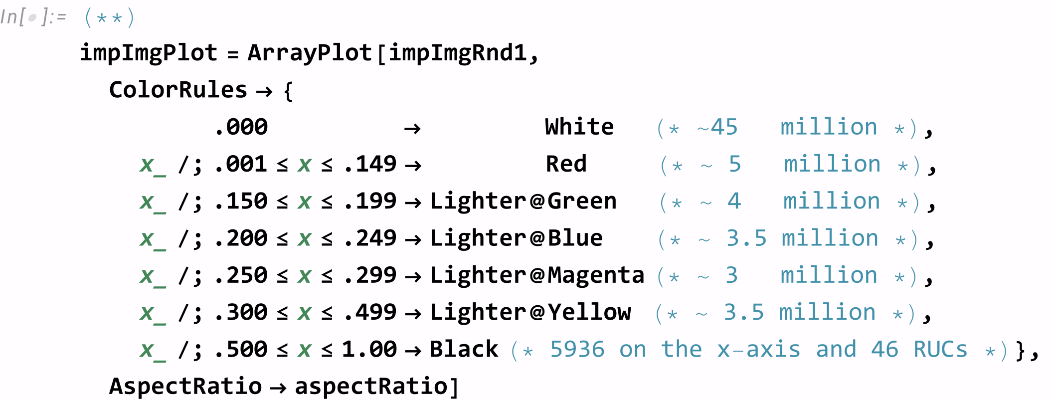
The roots are complex valued (Real x-axis and Imaginary y-axis) with normalized Abs@binValue defining the color from 0 to 1. The ColorRules are as follows:
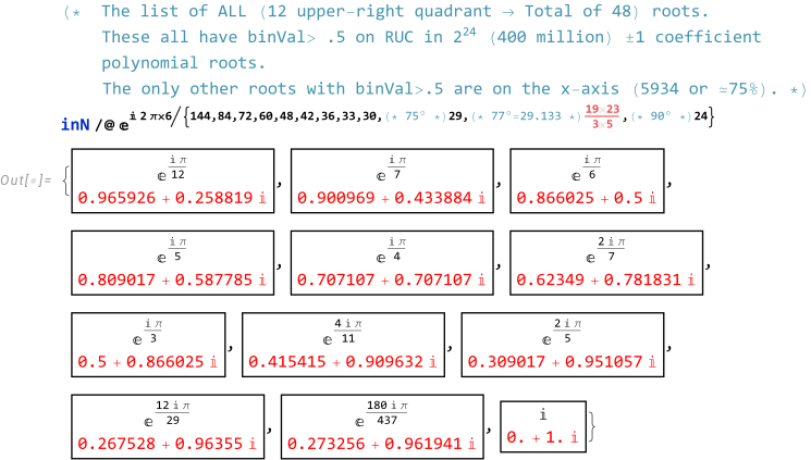
The analysis below provides more detail on the Roots-of-Unity Circle (RUC) at the center of the light yellow area. These are interesting in that there are 4 quadrants each with 12 roots that all have 1/2< Abs@binVal <1 at the center of holes.

There are 6 roots that sit in holes surrounded by zeros (i.e. 2π/{12,10,8,6,5,4}) and 6 roots in holes with surround values <1/2 (i.e. 2π/{24, 14, 7, 11/2, 29/6 (75°), 437/90 (77°)}). The only other binVal roots >1/2 are on the 1 pixel wide x-axis with 5936 of 8000 (~75%) from the x-y grid of 8000×8000 (64 million) bins which sum over each of the 224 (~16 million) roots-of-polynomials with -/+1 coefficients. The rest of the x-axis roots are 2020 bins equal to 0 and only 44 bins between 0 and 1/2).
The large table below shows 100 detail areas of “special” algorithmically selected locations from bin location Tally counts of 7732 unique binVals. About 50% of these occur in 2 to 4 (symmetric) locations with a binVal>1/2. The other 50% of the Tally counts have binVal<1/2 and tend to have 103 to 106 locations with all but 5980 (of 64 million) bins. This is made clear from the above MatrixPlots.

Each detail area shows a 400×400 ArrayPlot around the selected location and an 11×11 zoom-in of that Abs@binVal matrix with its ArrayPlot. They include the 48 RUC roots and 12 x-axis roots with binVal>1/2, and 40 off-axis roots with ~2/3 bins of zero and 1/3 with binVal<1/2. This off-axis list includes one set of 4 quadrant roots that is a proper hole (in the 4 yellow rings located just above/below the bottom/top apex in the full image or 10-14th from the bottom in the detail list below). The other 9×4 roots are what I call “pseudo-holes” that have no enclosed high central binVal.
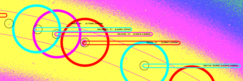
Zoom-in of detail in the upper-right quadrant RUC root values – click SVG to create another tab and zoom in your browser.

The annotated upper-right quadrant of the SVG image has the RUC roots ringed in colors (shown in the zoom-in graphic above) with large colored rings assigned by their binVal. Annotated rings with binVal>1/2 are cyan, magenta, and red. The binVal<1/2 are yellow, orange, or blue rings. The smaller black ring is what is visible in the 11×11 MatrixPlots below. To the right is the text with the angle at which the root is located.

FYI – The color scheme on these detail zoom MatrixPlots are set to the default in order to maximize and highlight the numeric differences, so they don’t match the ColorRules in the large 8000×8000 MatrixPlot at the top of the page.

Click the image below to see this SVG and zoom further.

Detail areas of special roots with a 1000×1000 ArrayPlot and an 11×11 zoom of the Abs root values and its ArrayPlot

Improved SVG E8 Petrie and Hexagonal Triality Representations

Stay tuned for more images. I think I will use this post to place my more beautiful works!

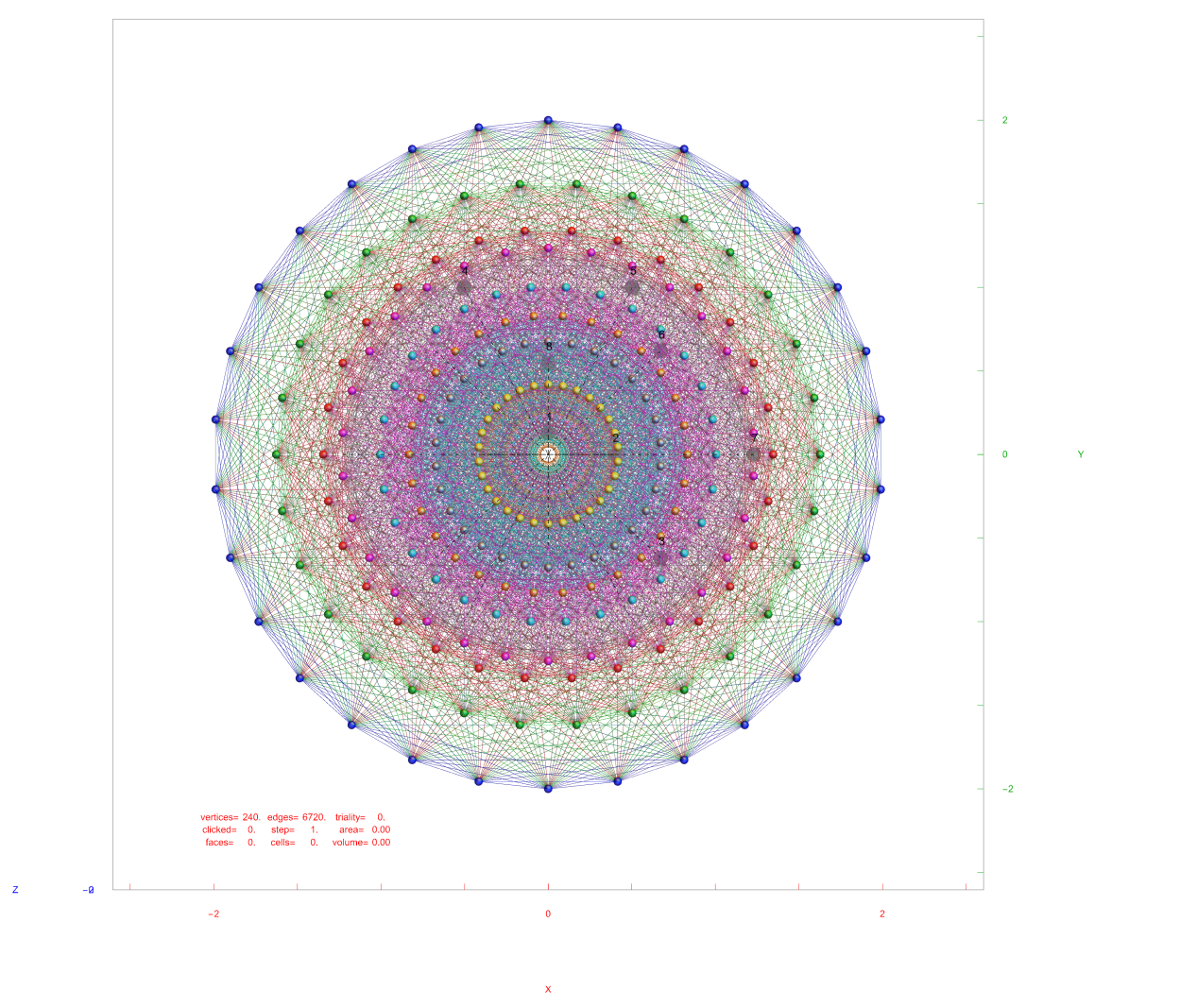
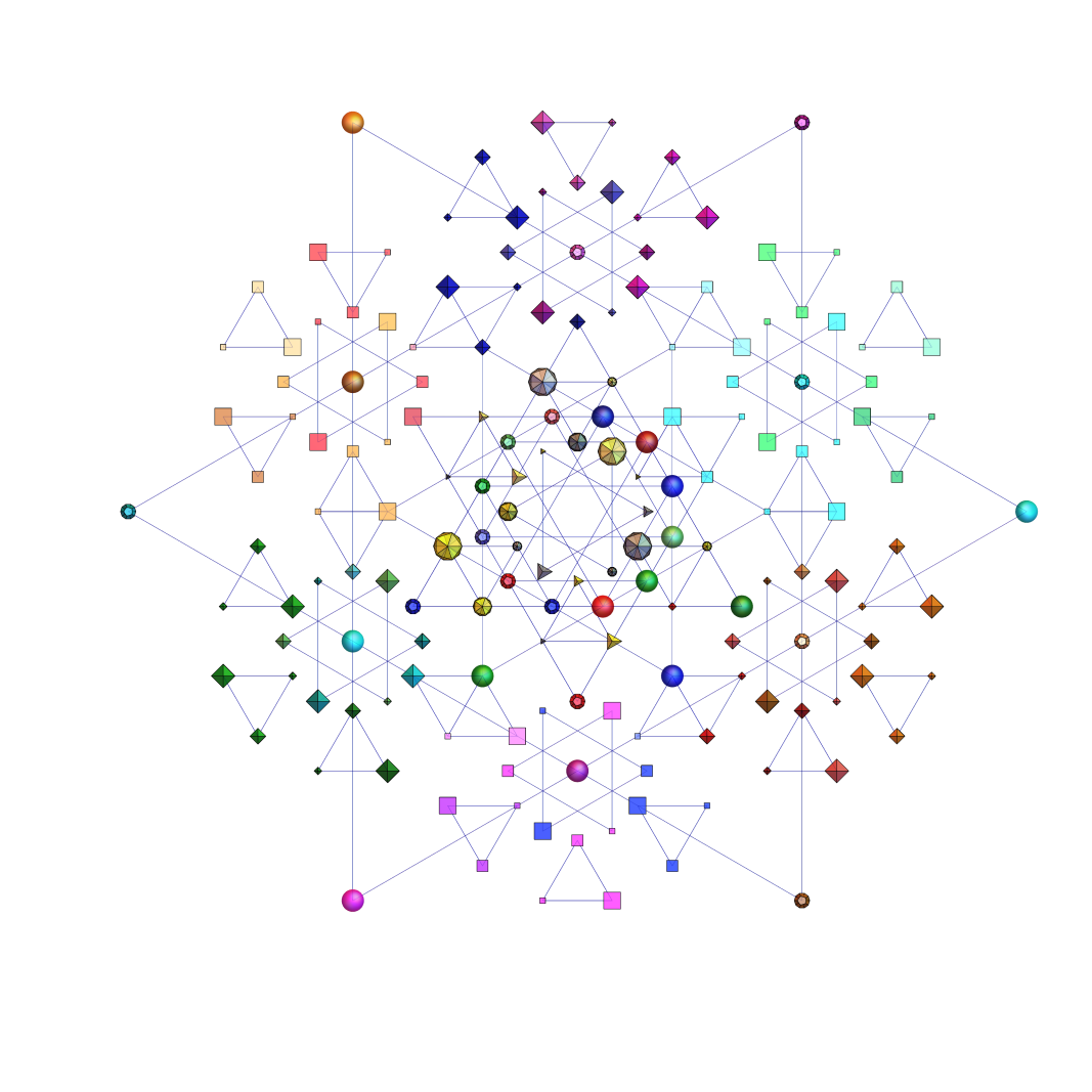
E8 in Petrie projection with 3D theoretically assigned physics particles

These use a better combination of specularity and opacity with both math and physics (theoretical assigned) 3D vertices. This is accomplished by actually projecting into 3D but using only X-Y basis vectors with Z={0,0,0,0,0,0,0,0} and the (virtual) camera at XYZ={0,0,}.

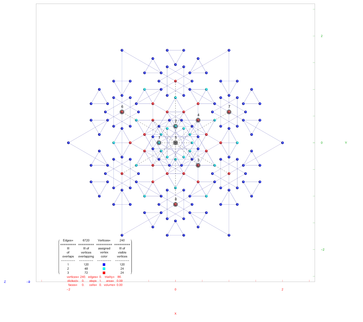
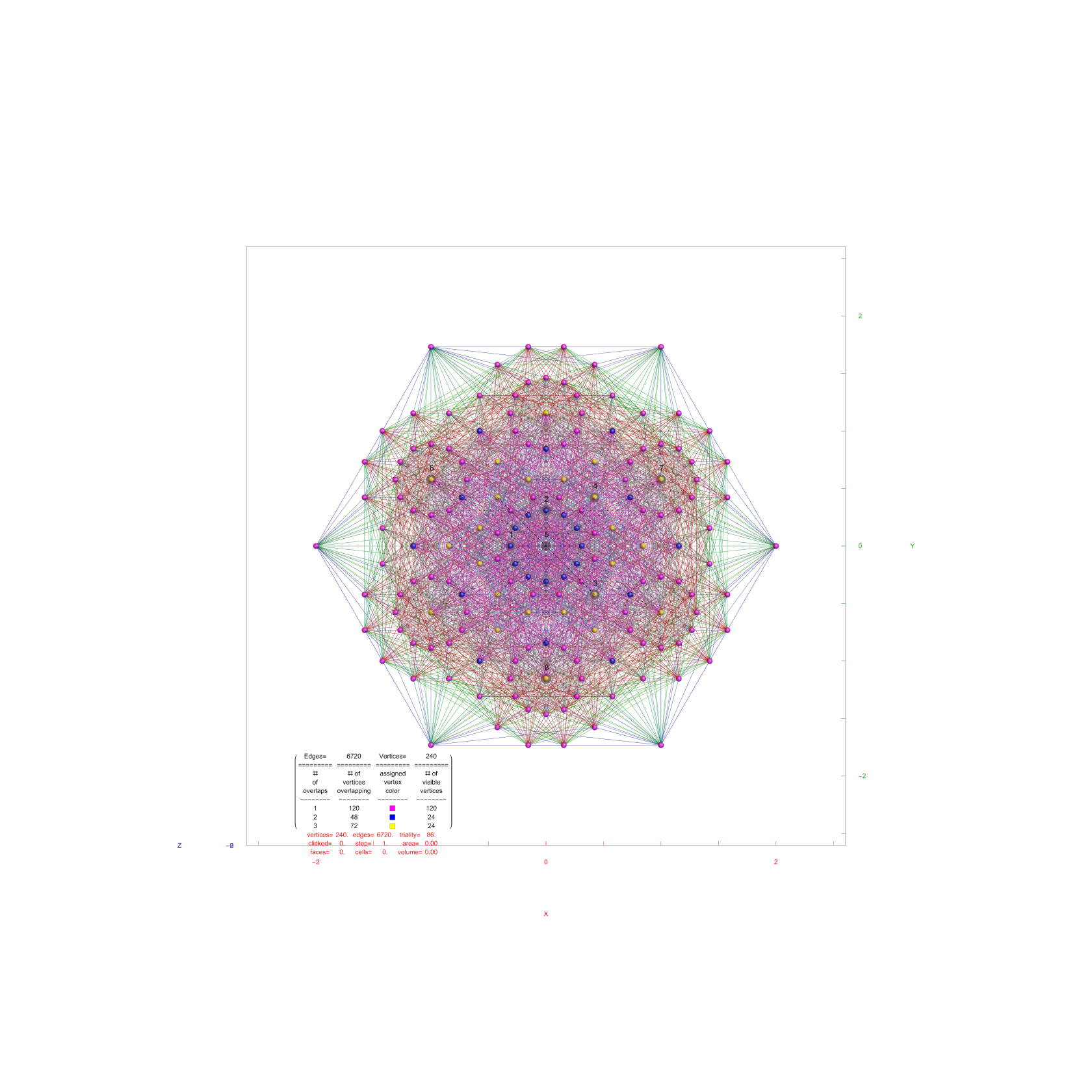
Some images use color coding for vertices that indicate overlaps (e.g. when in the spherical (math) vertices E8 hexagonal basis). The overlap number data may then be presented in the lower left. This data can be removed using SVG editors such as Inkscape.

Some images also show the 3D technical axes (basis) projection vectors as well as the vertex, edge, and other data. Also, bear in mind that the PNG images shown below (so they are visible in Google Images after being crawled) tend to show pixelation artifacts and can present with black background vs. white. The SVG presentation (obtained by clicking the embedded image link) will be correct and the transparent background can be modified easily (e.g. with Inkscape).

Please note, these are provided under Creative Commons CC BY-SA 4.0 Attribution-ShareAlike 4.0 International license, so if you use them please cite me at this site (or me on the Wikipedia (WP) article or WP commons source):

Below is the well known PR photo for E8 in Petrie projection with basis vector axes and data presented (click the image for the downloadable SVG):

E8 in Petrie projection with axes and other data

Below is the E8 hexagonal (aka. as the “E6/D4 Mox [6]” in Wikipedia) projection:

E8 hexagonal (aka. as the “E6/D4 Mox [6]” basis in Wikipedia) projection

The E8 hexagonal with the 3D assigned theoretical physics vertices:

E8 with the 3D assigned theoretical physics vertices in hexagonal projection

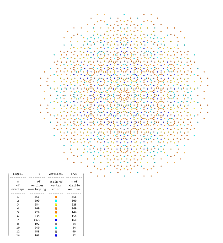
The E8 hexagonal projection with 6720 edges:

E8 with edges in hexagonal projection

The Rectified E8 in hexagonal projection with 6720 vertices:

Rectified E8 with edges in hexagonal projection

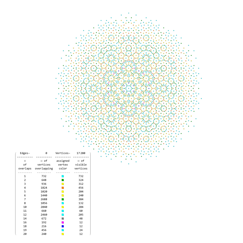
E8142 in hexagonal projection with 17280 vertices:

E8142 in hexagonal projection

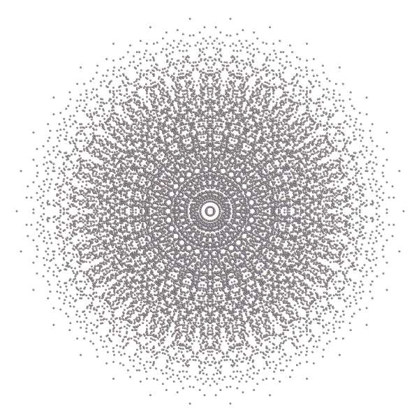
E8142 in Petrie projection with 17280 vertices:

E8142 in Petrie projection

The periodic table with orbitals in 2D:

The periodic table with orbitals in 2D

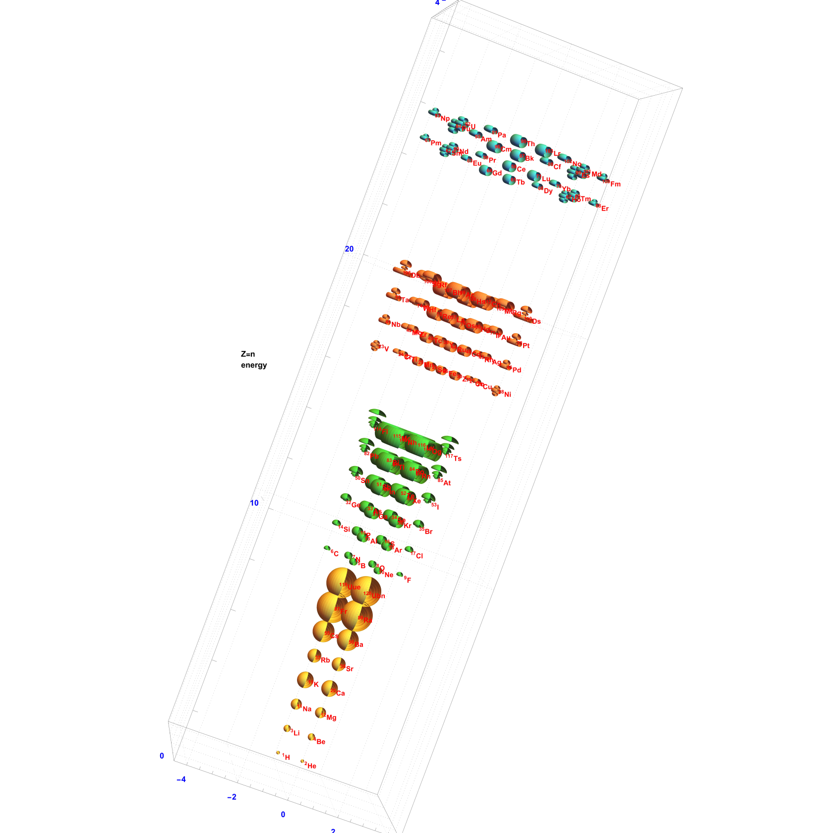
The periodic table with orbitals in 3D:

The periodic table with orbitals in 3D

Kneser neighborhood graph of Niemeier lattices with associated Mathematica Notebook here:

Kneser neighborhood graph of Niemeier lattices with associated Mathematica Notebook here.

The E8 subgroup tree:

E8 Subgroup Tree with associated Mathematica Notebook here.

Riemann Zeta function zeros:

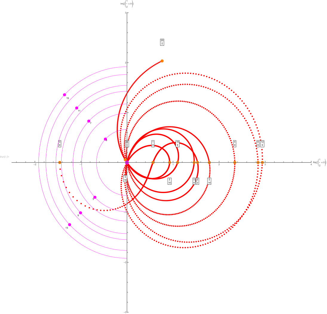
This is a polar plot of the first 20 non-trivial Riemann zeta function zeros (including Gram points along the critical line ζ(1/2+it) for real values of running from 0 to 50. The consecutive zeros have 50 red plot points between each with zeros identified by magenta concentric rings (scaled to show the relative distance between their values of t).
All roots of polynomials up to 224 (~16.7 million) with +/-1 coefficients.

E8 and H4 Gram Matrix Visualizations

Beautiful MatrixPlot’s of E8 and H4.

This is not the typical E8 Gram matrix representation as the Cartan matrix using only the simple roots (shown at the end of this post).

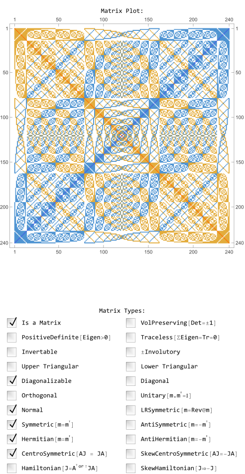
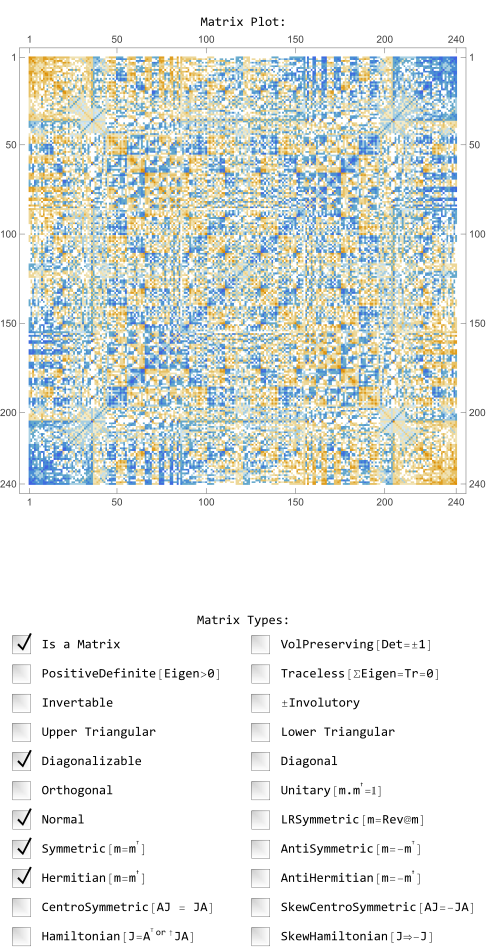
It uses all 240 E8 vertices (+120/-120 roots) of the E8 Split Real Even (SRE) vertices to produce the Gram matrix (with vertices sorted in simple numeric order):

Full E8 Split Real Even (SRE) vertex Gram matrix in vertex numeric sort order

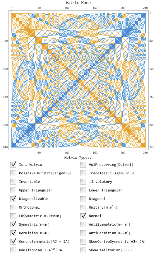
The same 240 E8 vertices (+120/-120 roots) below are sorted by the 9th row of the binary structure Pascal Triangle, excluding the 2nd & 2nd to last entries of -/+ 8 (i.e. {-1,-8,-28,-56,70=(-35/35),56,28,8,1}, where the 112 integer D8 are -56/56 and the 128 half-integer BC8 are {-1,-28,-35,35,28,1}).

Full E8 Split Real Even (SRE) vertex E8 Gram matrix in Pascal Triangle order

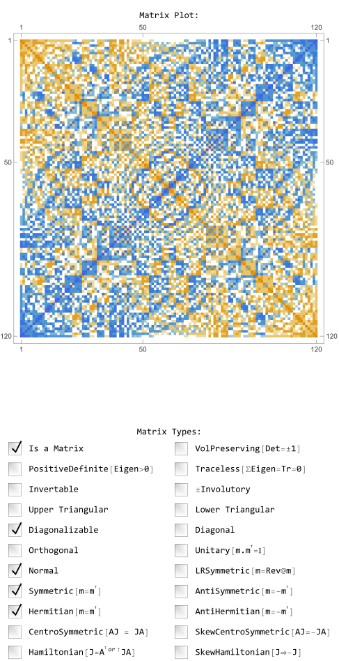
As above, but with H4+H4φ 8D Gram matrix created using the dot product of E8 against the 8×8 E8 to H4 folding matrix U:

H4+H4φ 8D Gram matrix

Now with only the H4φ 4D Gram matrix created as 120 H4 4D vertices:

H4φ 4D Gram matrix

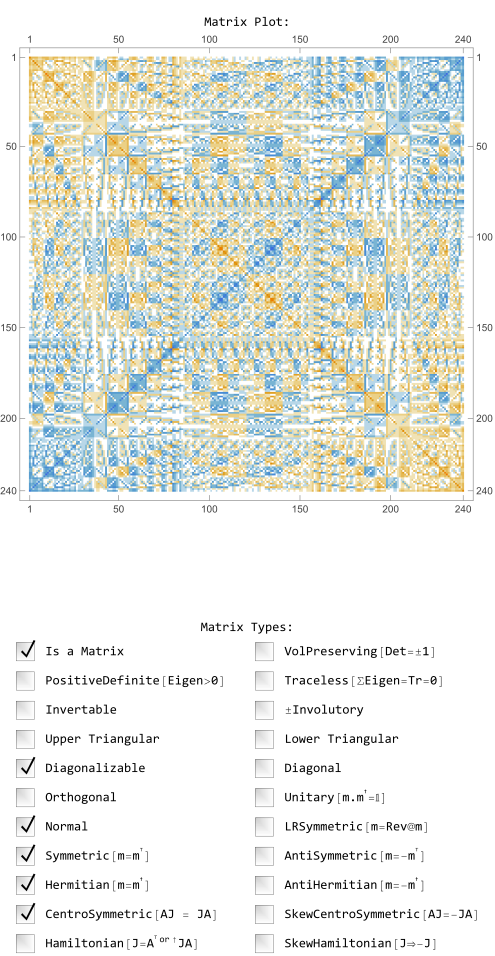
Compare this to the Gram matrix using the root weights of E8 (in Pascal triangle order vs. sorted into root and/or weight order):

E8 Gram Weights (in Pascal Triangle order)

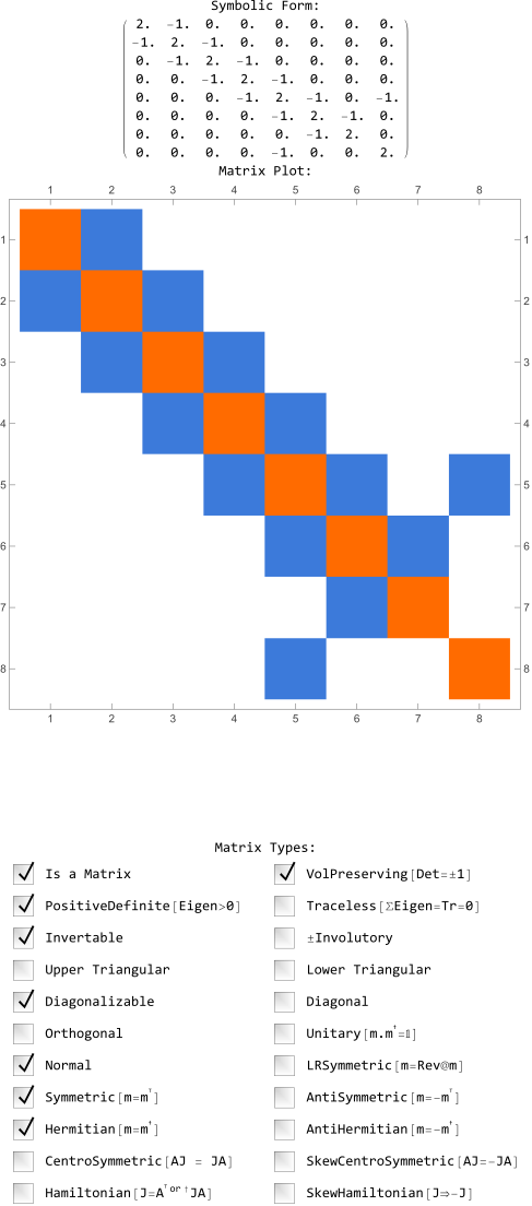
Then compare to the Cartan matrix produced as the Gram matrix of only the 8 E8 simple roots:

E8 Cartan matrix from 8 simple roots

Info about my creative work: The Universe, Math, Physics, & Art

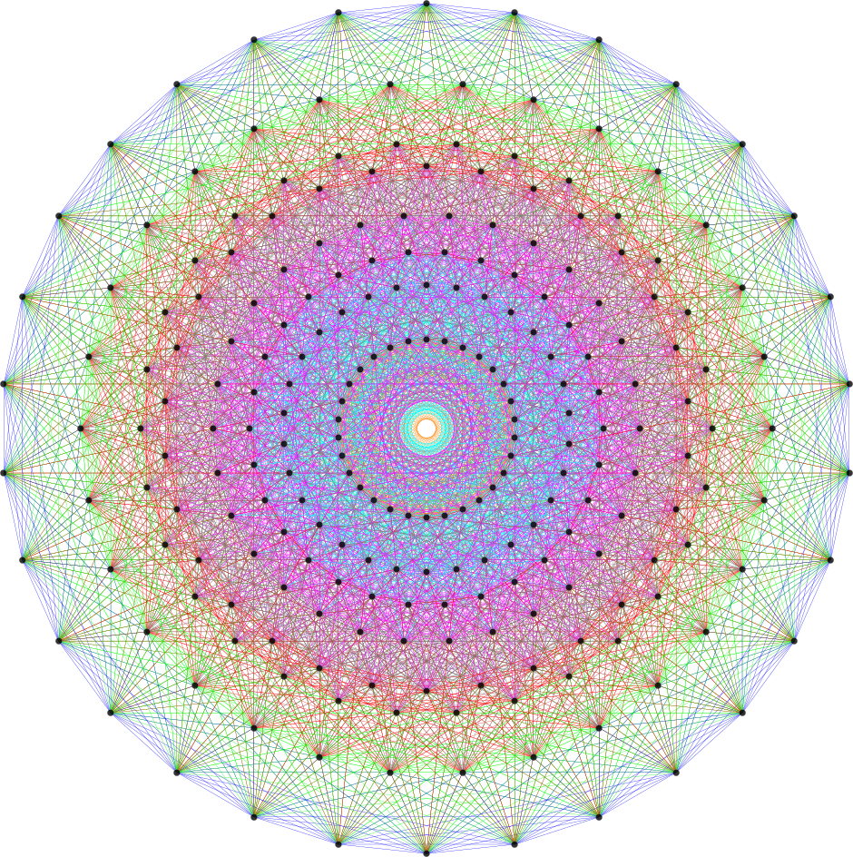
I think the most well-known (2D) image I’ve created so far (above) is found on Wikipedia’s (WP) math/geometry pages. It is what has been called the Public Relations (PR) or publicity photo for E8, which is an 8D (or 248 dimensional as the math guys count it) geometric object. It has been used in books, papers, math/science conference promotional materials, etc. That WP page also has what many used to consider “uninteresting” – my 3D versions of the same object. E8 is used in various theories to understand how the Universe operates way below the atomic level (i.e. the quantum stuff). I think it is responsible for what I call the shape of the Universe. As others have said, “who knew the Universe had a shape?”

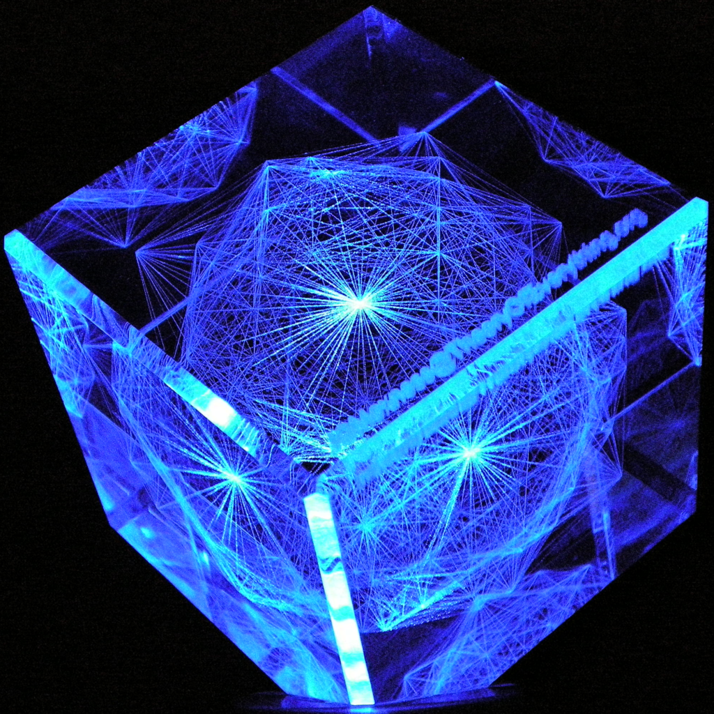
In (very) layman’s terms, that 2D image of E8 looks sort-of-like how the lowly 4D Tesseract cube would look if it grew up into an 8D object, but a bit more interesting. The Tesseract was made (more) popular in the modern Avengers movies. In 2015 before I had ever seen any of those movies, I created a laser etched 3D projection of E8 within a jewel cut optical crystal cube and put a photo of that object lit from below by a blue LED on my website’s main homepage. Someone mentioned the resemblance and I was surprised at the likeness, motivating me to go see the movies.

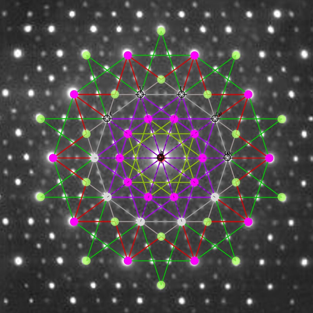
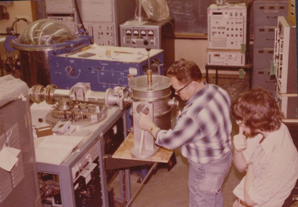
Another of my more notable math/physics images has to do with the discovery of QuasiCrystals made by a guy, Dan Shechtman, who was ostracized from academia for the “impossible” idea of crystals having rotational symmetries beyond 2,3,4 and 6. He is now a Nobel Laureate. The WP image above is on that QuasiCrystal page as an overlay of part of E8 projected over a picture made from shooting a beam of x-rays at an icosahedral Ho-Mg-Zn quasicrystal.  I didn’t actually do that experiment with the x-ray beams, but I did similar ones in my college days on a particle accelerator called the Cockroft-Walton Kevatron – see below for a picture of me (the one with the beard ;–)  in the physics lab assembling a moon dust experiment. One of the professors had gotten the accelerator out of Germany after having worked on the Manhattan project.

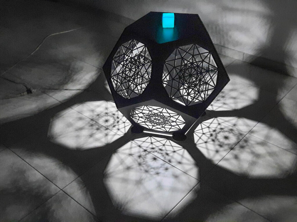
E8 and its 4D children, the 600-cell and 120-cell (pages on which I have some work, amongst others) and its grandkids (2 of the 3D 5 Platonic Solids, one of which is the 3D version of the 2D Pentagon) are all related to the Fibonacci numbers and the Golden Ratio. So that kind of explains why most of my 2D art, 3D objects and sculptures (e.g. furniture like the dodecahedron table below), and 4D youtube animations all use the Golden Ratio theme.

Greg Moxness, Tucson AZ

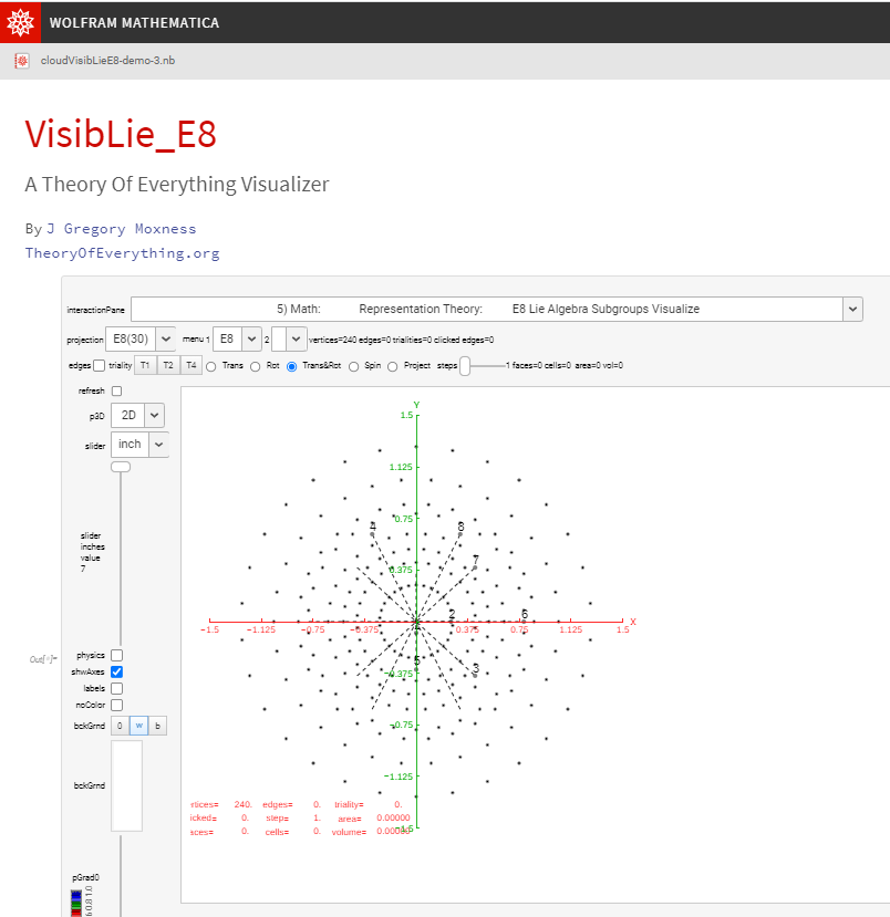
Cloud Based VisibLie_E8 Demonstration

The cloud deployments don’t have all the needed features as the fully licensed Mathematica notebooks, so I included a few of the panes that seem to work for the most part. Some 3D and animation features won’t work, but it is a start. Bear in mind that the response time is slow.

Link to the demonstration.

A Theory of Everything Visualizer, with links to free Cloud based Interactive Demonstrations:

1) Math: Chaos/Fibr/Fractal/Surface: Navier Stokes/Hopf/MandelBulb/Klein

2) Math: Number Theory: Mod 2-9 Pascal and Sierpinski Triangle

3) Math: Geometric Calculus: Octonion Fano Plane-Cubic Visualize

4) Math: Group Theory: Dynkin Diagram Algebra Create

5) Math: Representation Theory: E8 Lie Algebra Subgroups Visualize

6) Physics: Quantum Elements: Fundamental Quantum Element Select

7) Physics: Particle Theory: CKM(q)-PMNS(ν) Mixing_CPT Unitarity

8) Physics: Hadronic Elements: Composite Quark-Gluon Select Decays

9) Physics: Relativistic Cosmology: N-Body Bohmian GR-QM Simulation

10) Chemistry: Atomic Elements: 4D Periodic Table Element Select

11) Chemistry: Molecular Crystallography: 4D Molecule Visualization Select

12) Biology: Genetic Crystallography: 4D Protein/DNA/RNA E8-H4 Folding

13) Biology: Human Neurology: OrchOR Quantum Consciousness

14) Psychology: Music Theory & Cognition: Chords, Lambdoma, CA MIDI,& Tori

15) Sociology: Theological Number Theory: Ancient Sacred Text Gematria

16) CompSci: Quantum Computing: Poincare-Bloch Sphere/Qubit Fourier

17) CompSci: Artificial Intelligence: 3D Conway’s Game Of Life

18) CompSci: Human/Machine Interfaces: nD Human Machine Interface

The free Wolfram CDF Player v. 13 works with my VisibLie E8 ToE demonstration on Win10

In case you’re interested, I just verified the demo works on the free Mathematica CDF player v.13 for Win10.

Just go to https://www.wolfram.com/player/ install, download and open the app:

https://theoryofeverything.org/TOE/JGM/ToE_Demonstration.nb

There is a ton of other cool interactive stuff in there. FYI – Some features don’t work without a full Mathematica license.

Enjoy.