Tag Archives: Dynkin

My latest paper on E8, the H4 folding matrix, and integration with octonions and GraviGUT physics models.

The full paper with appendix can be found on this site, or w/o appendix on viXra. (13 pages, 14 figures, 20Mb). The 22 page appendix contains the E8 algebra roots, Hasse diagram, and a complete integrated E8-particle-octonion list.

E82DPetriePhysics

Abstract:
This paper will present various techniques for visualizing a split real even E8 representation in 2 and 3 dimensions using an E8 to H4 folding matrix. This matrix is shown to be useful in providing direct relationships between E8 and the lower dimensional Dynkin and Coxeter-Dynkin geometries contained within it, geometries that are visualized in the form of real and virtual 3 dimensional objects. A direct linkage between E8, the folding matrix, fundamental physics particles in an extended Standard Model GraviGUT, quaternions, and octonions is introduced, and its importance is investigated and described.

If you would like to cite this, you can use this BibTex format if you like (remove the LaTex href tag structure if you don’t use the hyperref package):


@article{Moxness2014:006,
title={{The 3D Visualization of E8 using an H4 Folding Matrix}},
author={Moxness, J. G.},
journal={href{http://vixra.org/abs/1411.0130}{www.vixra.org/abs/1411.0130}},
year={2014},
month = nov,
adsurl={http://vixra.org/abs/1411.0130}
}

paper

Hyperbolic Dynkin #136 Detail

In followup to John Baez’ G+ thread on Hyperbolic Dynkin diagrams, specifically on the only rank 4 compact symmetrizable diagram 136, I used my “VisibLie” notebook (which includes the “SuperLie” package for analyzing Lie Algebras) to get the following information:

H136_detail3

Using the “SimpLie” Google Code OpenSource software, we get Hasse diagram of:
Projection of H136
Symmetrized Cartan matrix:
1 -1 0 -1/2
-1 2 -1 0
0 -1 2 -1
-1/2 0 -1 1

One possible set of basis vectors for this is:
srH136={{0,2,0,0},{0,-1,1,0},{0,0,-1,1},{Sqrt[-7],-1,-1,-3}};

with 4D angles between each node of:
{{1->2,135.},{2->3,120.},{3->4,135.},{4->1,120.},{1->3,90.},{2->4,90.}}

Norm’d Length between nodes is:
{2, Sqrt[2], Sqrt[2], 2}

as visualized in 2D and 3D, with 42 vertices and 26 edges of Norm’d 4D length of 2 and 94 at Sqrt[2]:
H136_Lowe_projection7

H136_Lowe_projection8

JGM_ToE-now-21d

Mathematica MyToE on the Wolfram Cloud

I am playing around with the Wolfram Tweet-a-Program, and the Wolfram Language (i.e. Mathematica) on the Wolfram Cloud.

What’s really cool is that you can now interact with advanced math and HPC on your phone/tablet.

Here are a few results…
@Wolframtap

ByeDZ-oIgAA8tZz

ByzPbCqIQAAzUJq.png large

BTW – you will need a WolframID (and be logged into WolframCloud.com) to interact with these pages.

Octonions: The Fano Plane & Cubic

MTMcloud-Fano

Dynkin Diagrams

MTMcloud-Dynkin

E8 and Subgroup Projections

MTMcloud-E8

Particle Selector

MTMcloud-Particle

Hadron Builder

MTMcloud-Hadron

Navier-Stokes Chaos Theory, 6D Calabi-Yau and 3D/4D Surface visualizations

MTMcloud-Chaos

Solar System (from NBody Universe Simulator)

MTMcloud-NBody
4D Periodic Table

MTMcloud-Atom

Interactive Hasse Visualizations and StereoScopic viewing

Along with added options for Left-Right and Red-Cyan Anaglyph stereoscopic outputs on the left side control panel…

outE80a

outE80b

outAtom

outAtom-aa

outNBody_1

I’ve added Interactive Hasse Visualizations to the #2 Dynkin Demonstration Pane. There is now a checkbox for showing the detail root vector data and Hasse visualizations (instead of the default interactive Dynkin pane). This is done from an integration of SuperLie 2.07 by P. Grozman.

If you have a full licensed Mathematica, use ToE_Demonstration.nb. For use with the free CDF Player, use ToE_Demonstration.cdf or as an interactive web page.

D4_Hasse

C5_Hasse

F4_Hasse

E6_Hasse

E7_Hasse

E8_Hasse

outDynkin-1

outDynkin-2

E7-Hasse

E8 folding to H4+H4/φ

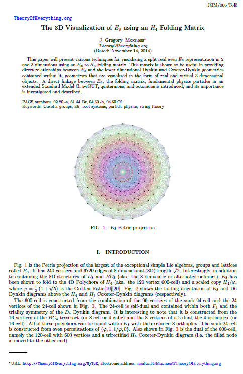
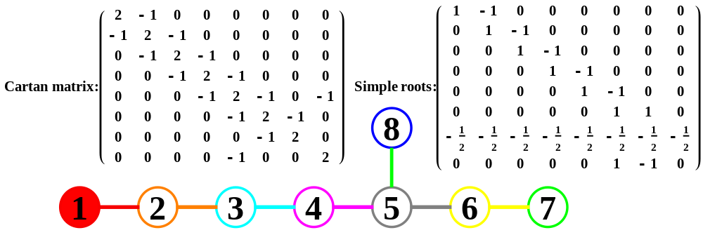
I found the rotation matrix that shows the E8 Dynkin diagram can indeed be folded to H4+H4/φ.

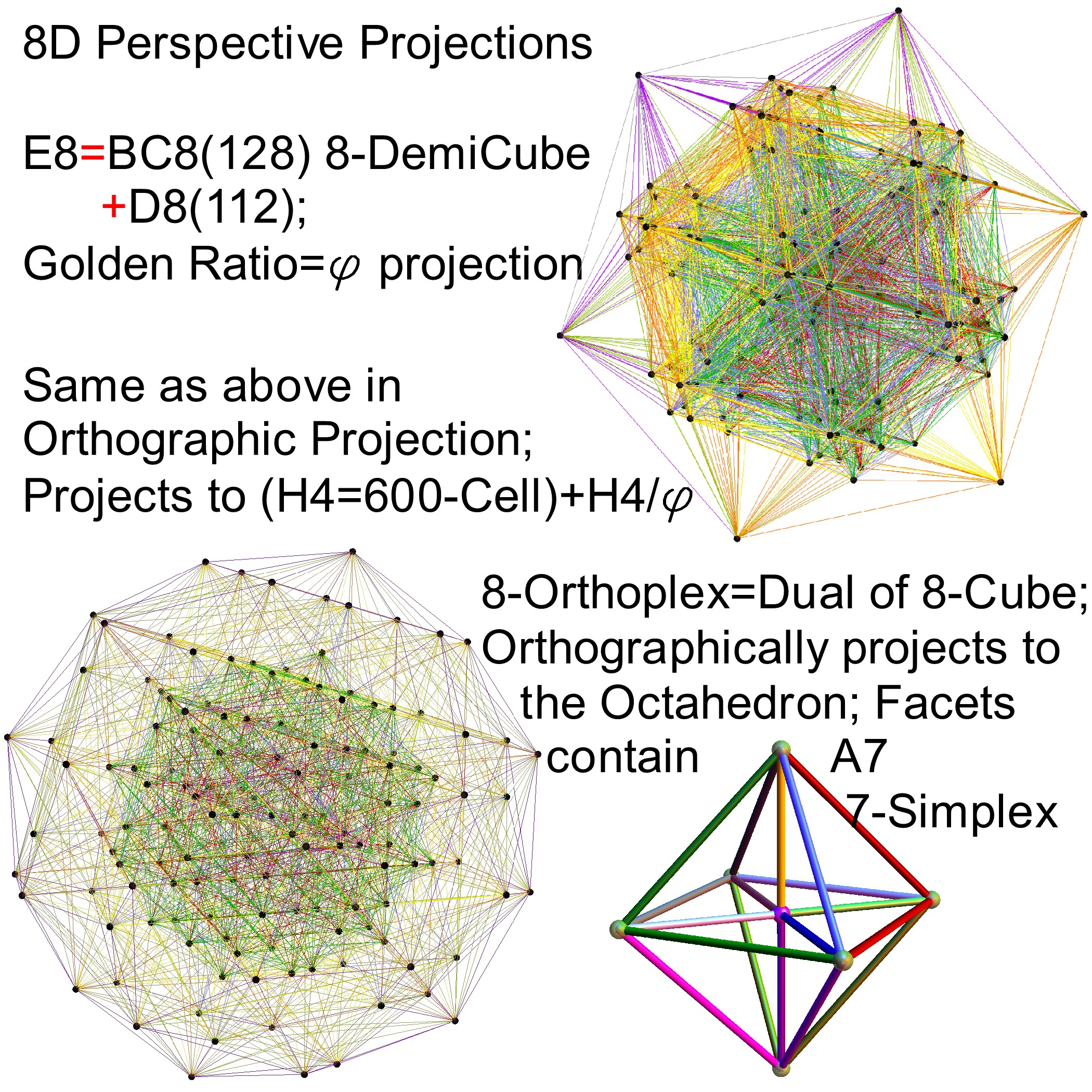
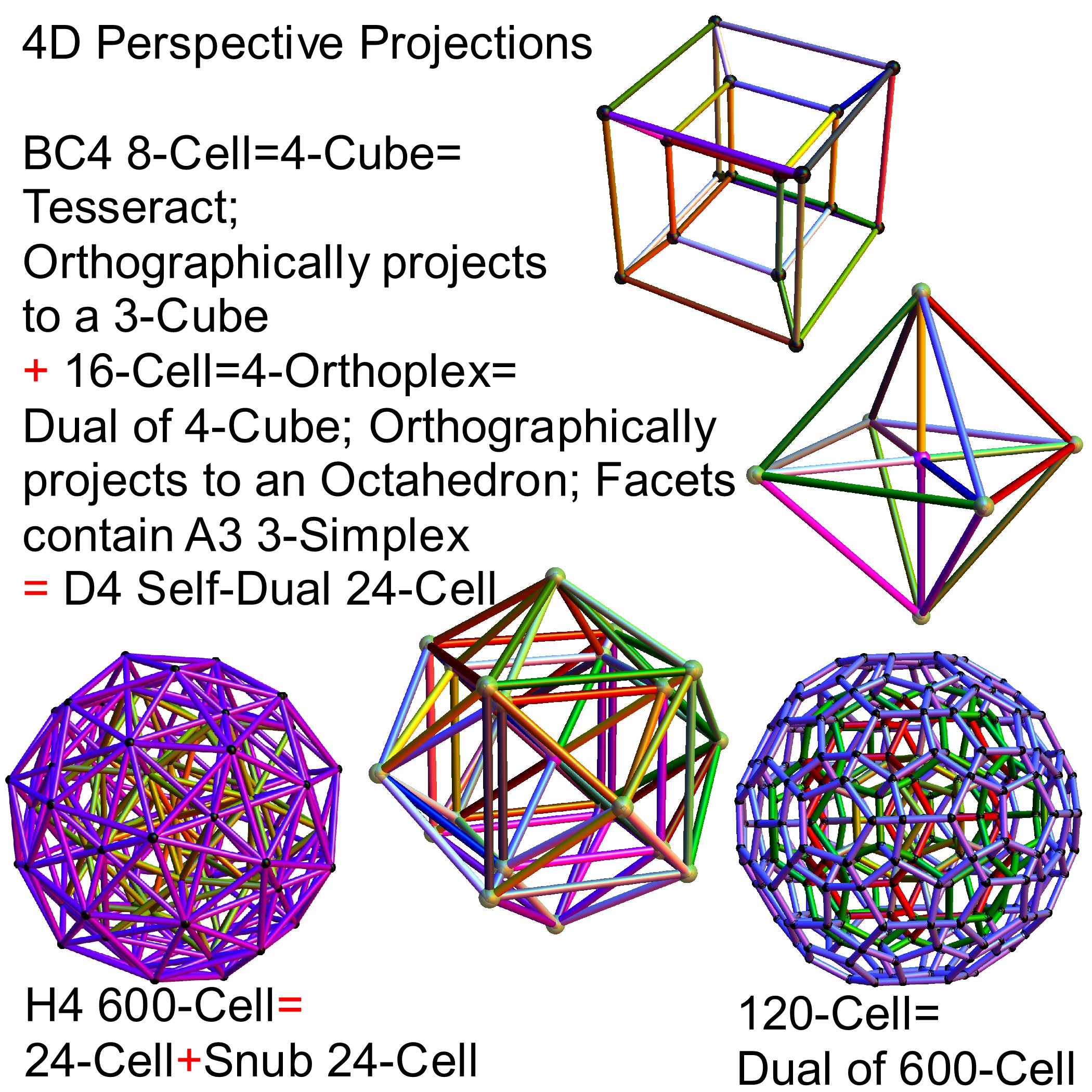
The H4 and its 120 vertices make up the 4D 600 Cell. It is made up of 96 vertices of the Snub 24-Cell and the 24 vertices of the 24-Cell=[16 vertex Tesseract=8-Cell and the 8 vertices of the 4-Orthoplex=16-Cell]).

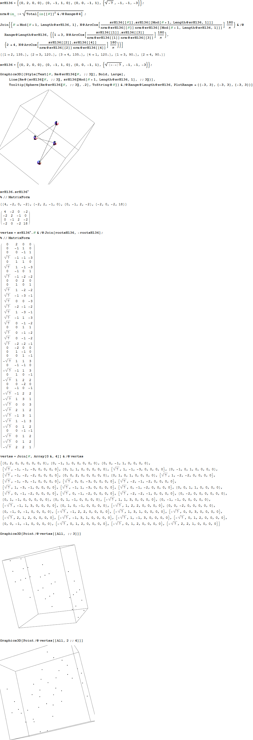
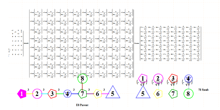
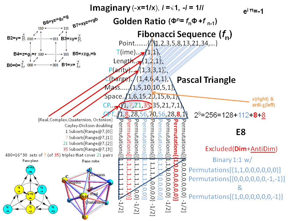
It can be generated from the 240 split real even E8 vertices using a 4×8 rotation matrix:
x = (1, φ, 0, -1, φ, 0, 0, 0)
y = (φ, 0, 1, φ, 0, -1, 0, 0)
z = (0, 1, φ, 0, -1, φ, 0, 0)
w = (0, 0, 0, 0, 0, 0, φ^2, 1/φ)

where φ=Golden Ratio=(1+Sqrt(5))/2

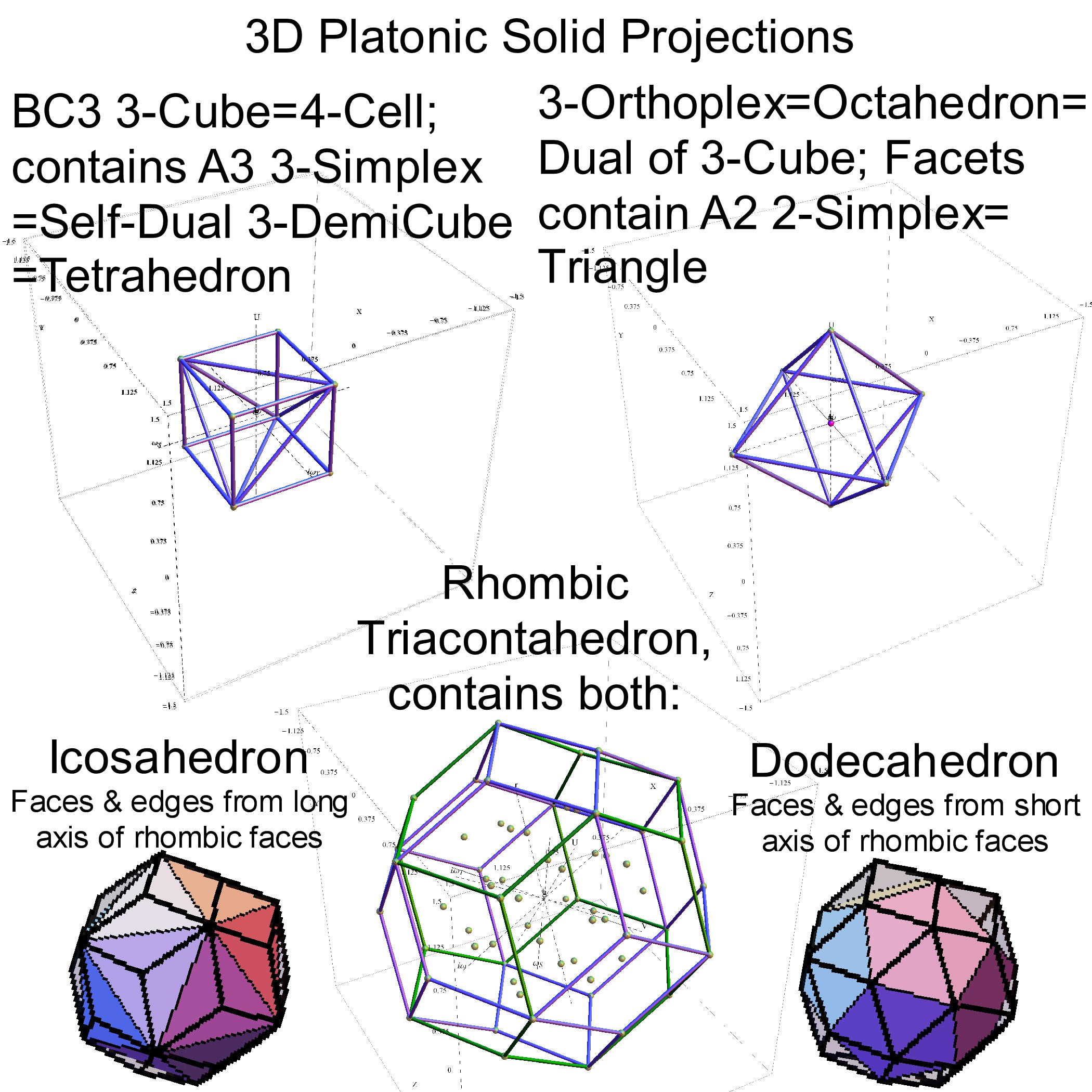
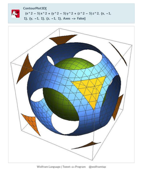
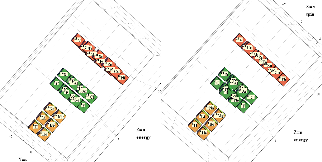
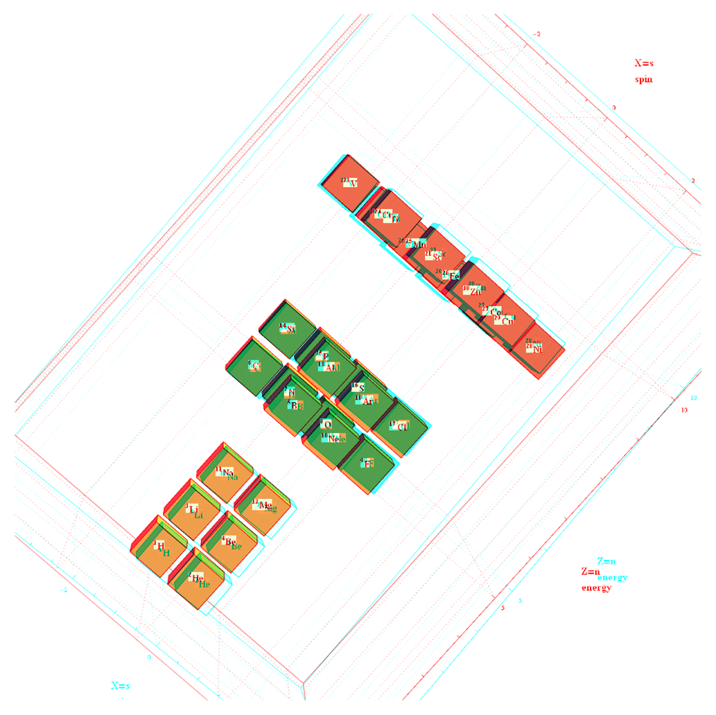
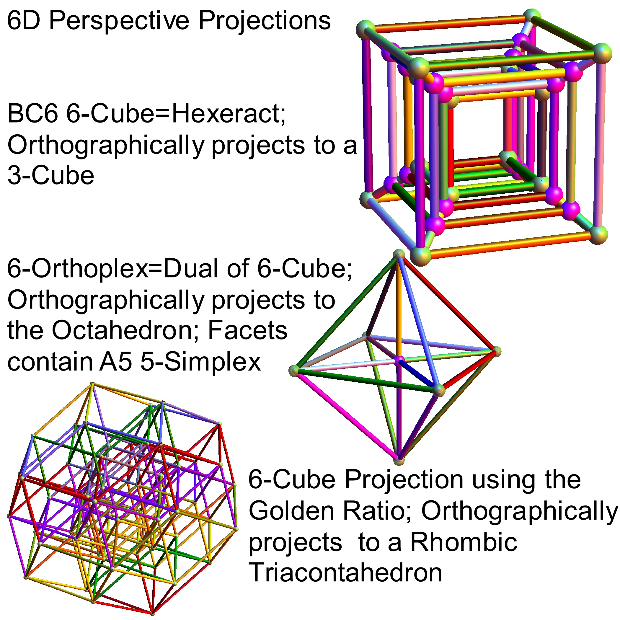
It is also interesting to note that the x, y, and z vectors project to a hull of the 3D Rhombic Triacontrahedron from the 6D 6 cube Hexaract (which then generates the hull of the Dodecahedron and Icosahedron Platonic solids).

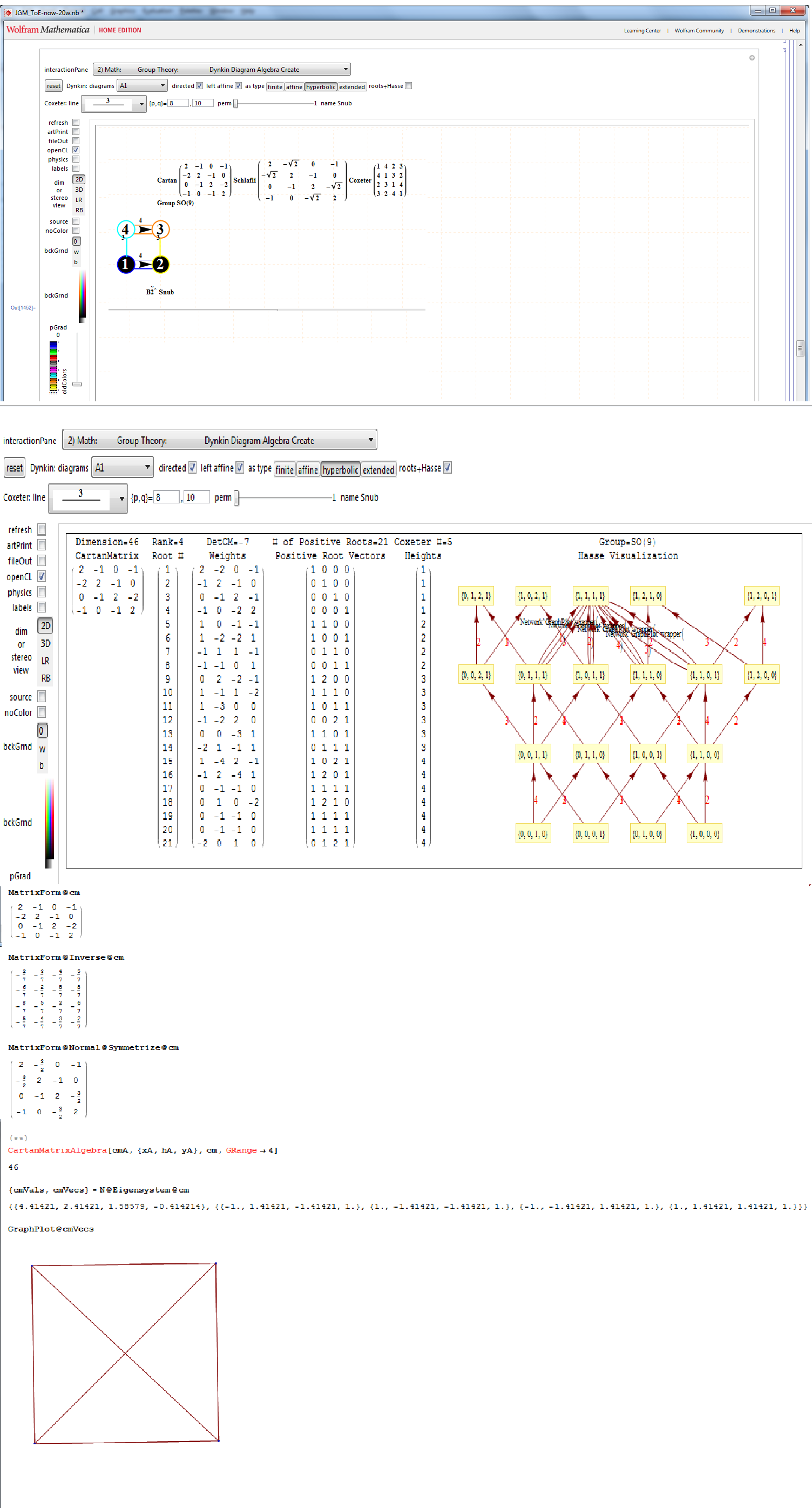
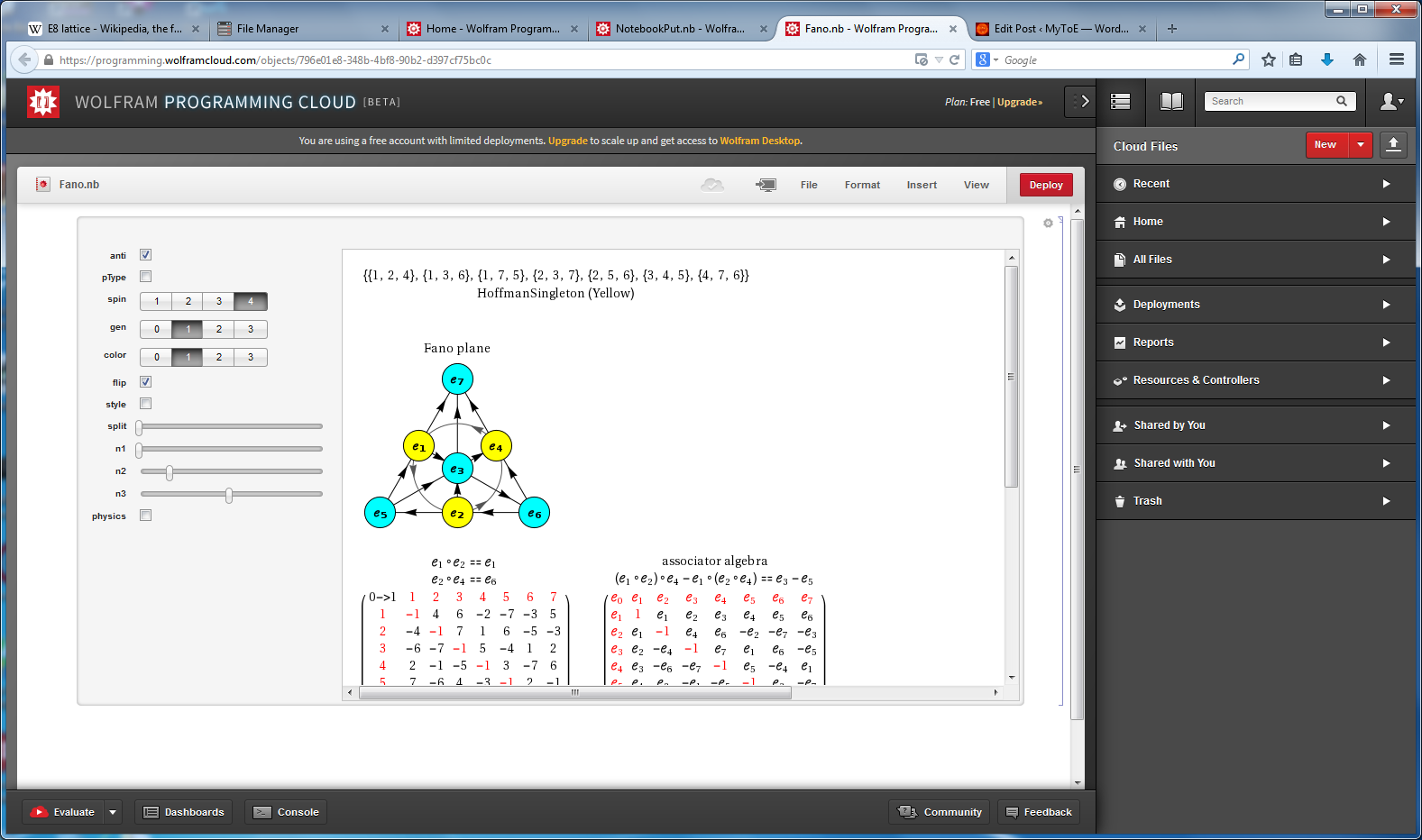
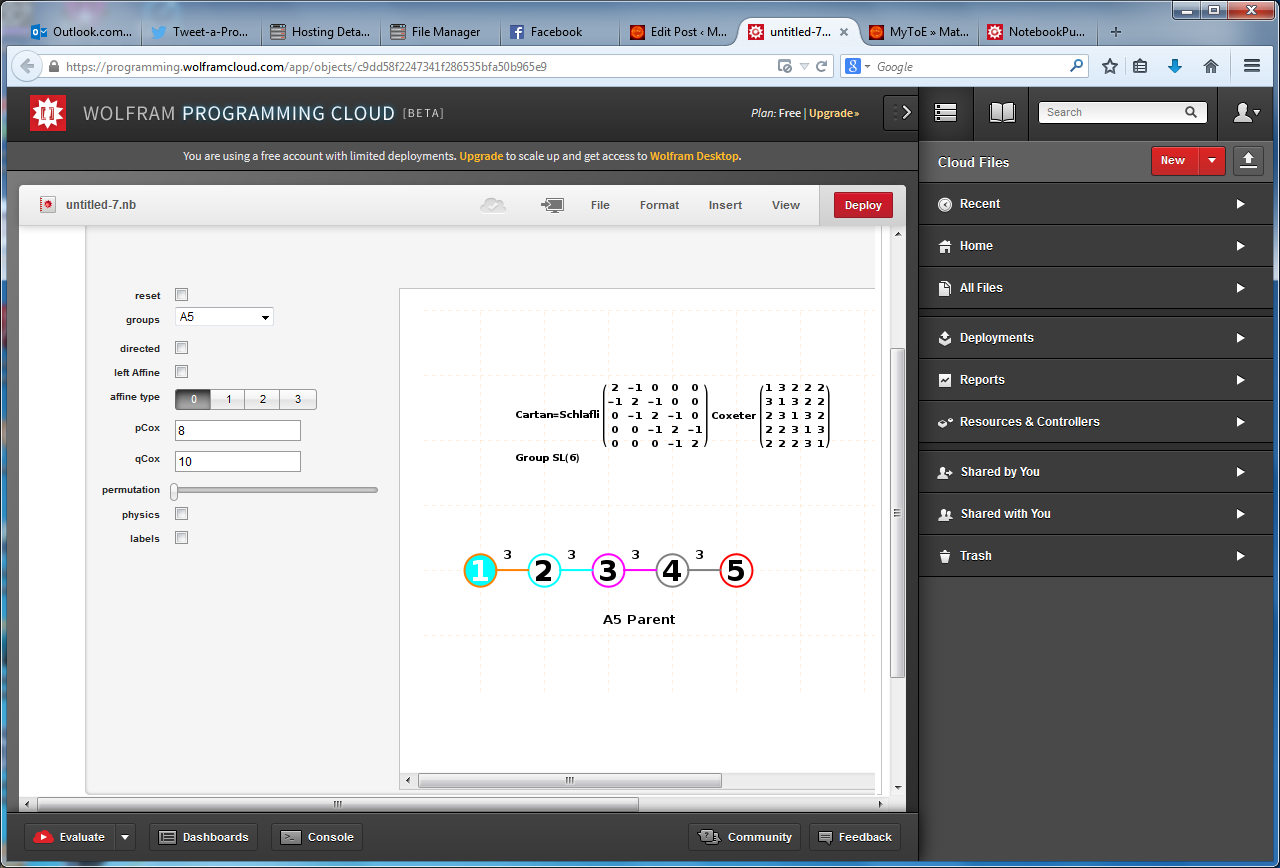
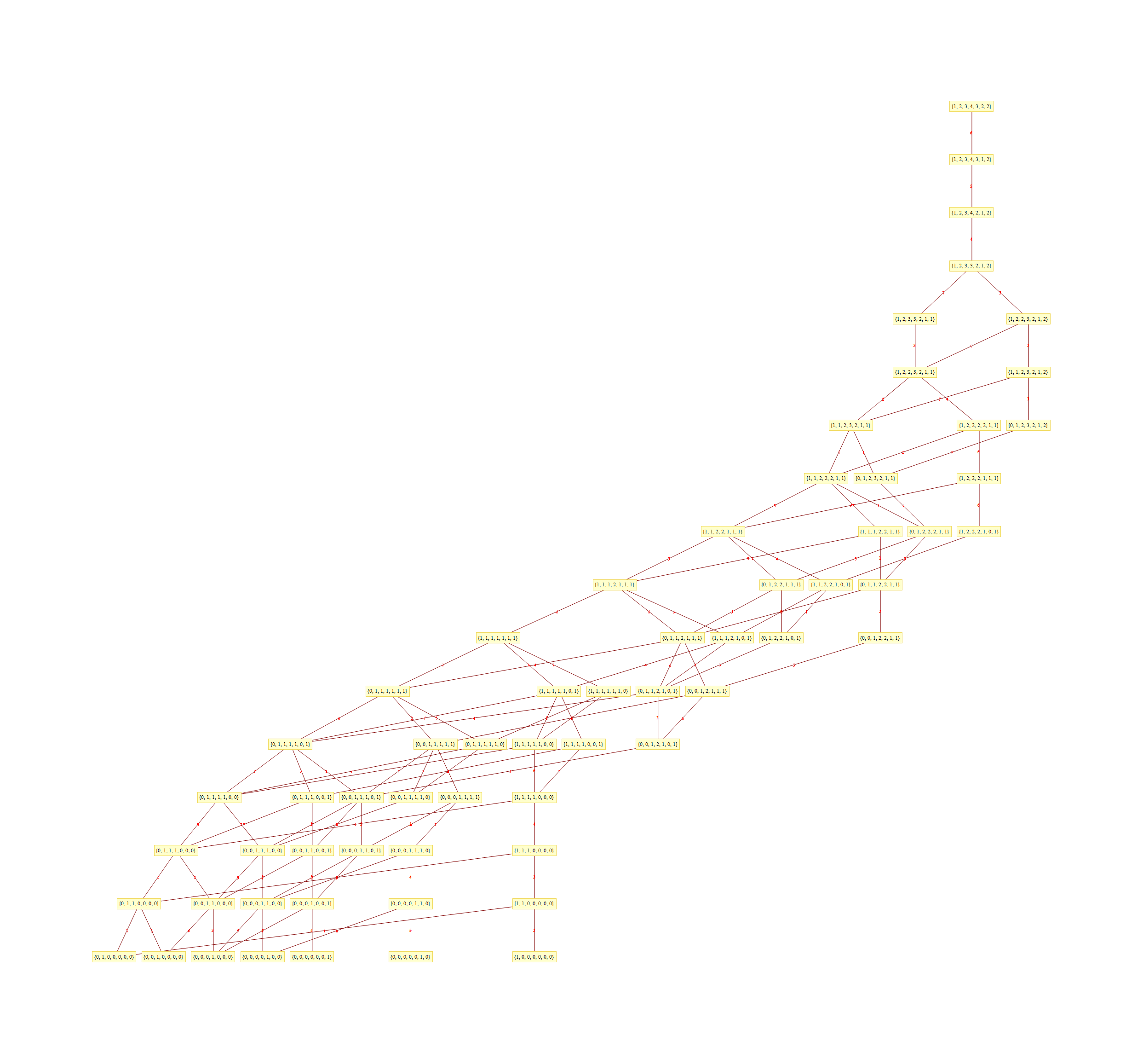
Here’s a look at the Dynkin Diagram folding of E8 to H4+H4/φ:

E8-H4-Fold

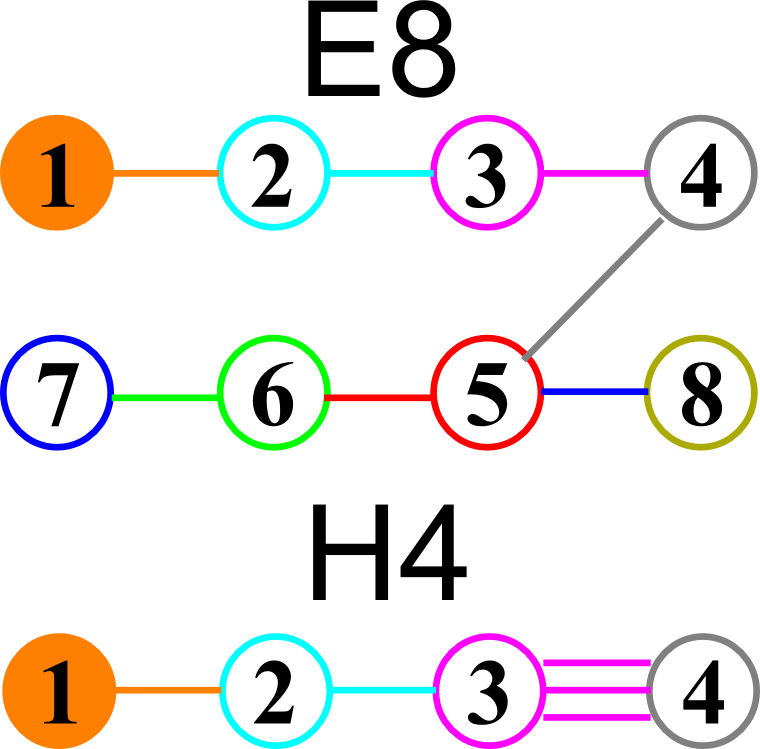
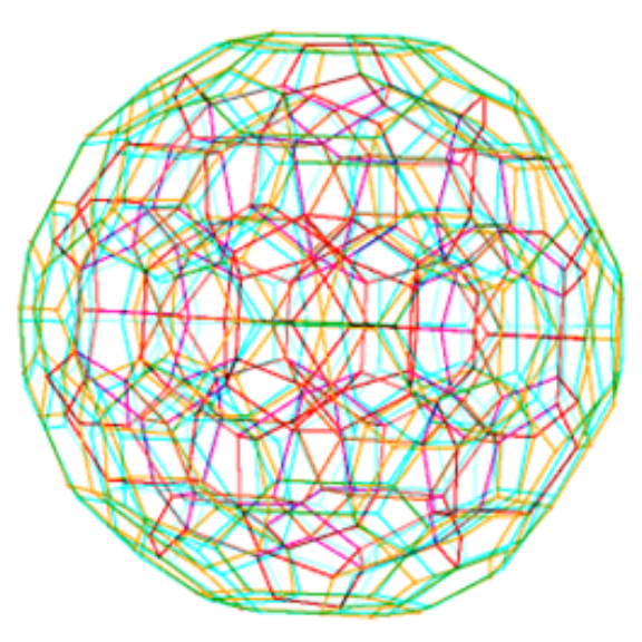
I find in folding from 8D to 4D, that the 6720 edge counts split into two sets of 3360 from E8’s 6720 length Sqrt(2), but the combined edges and vertices recreate the E8 petrie diagram perfectly.

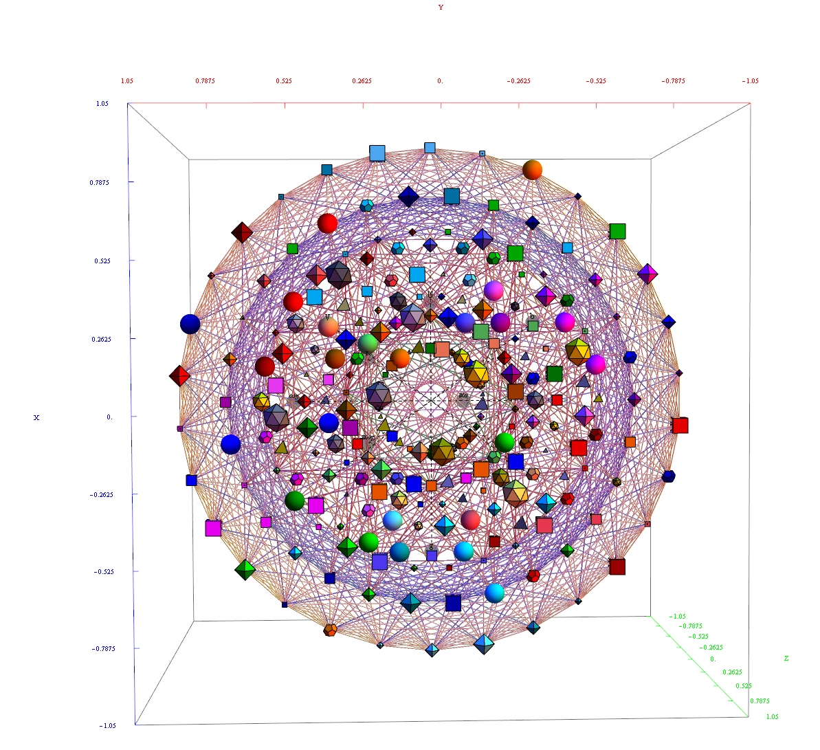
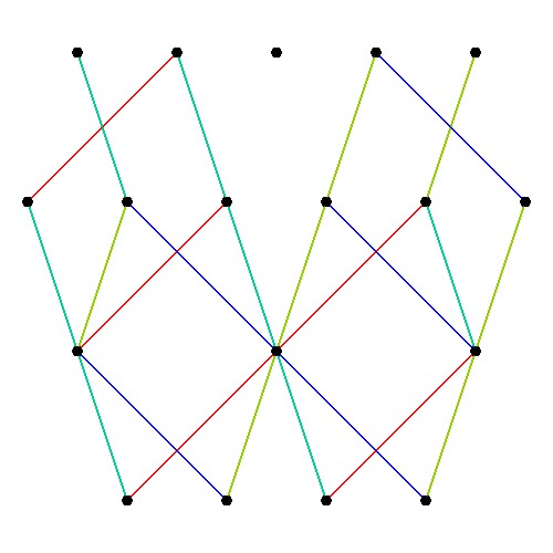
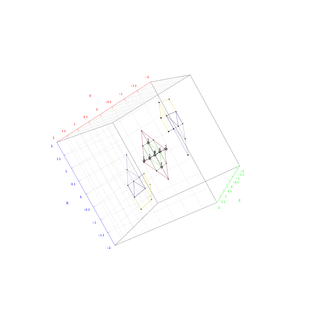
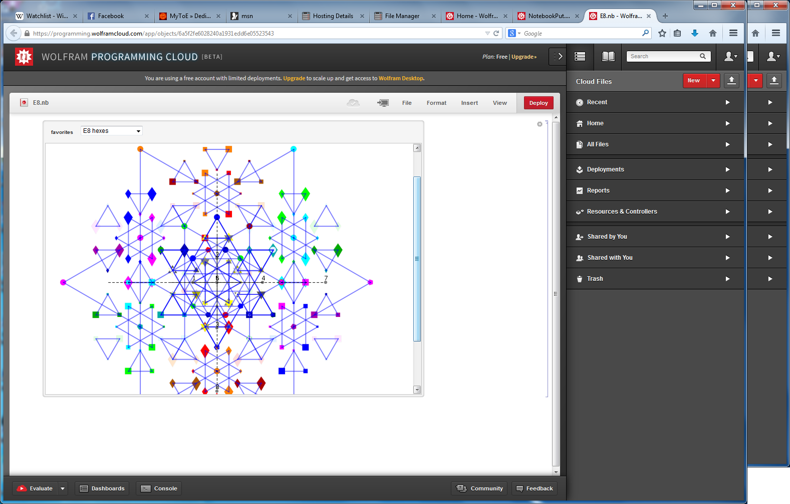
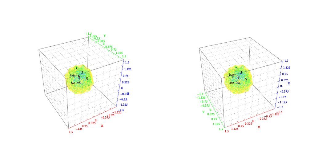
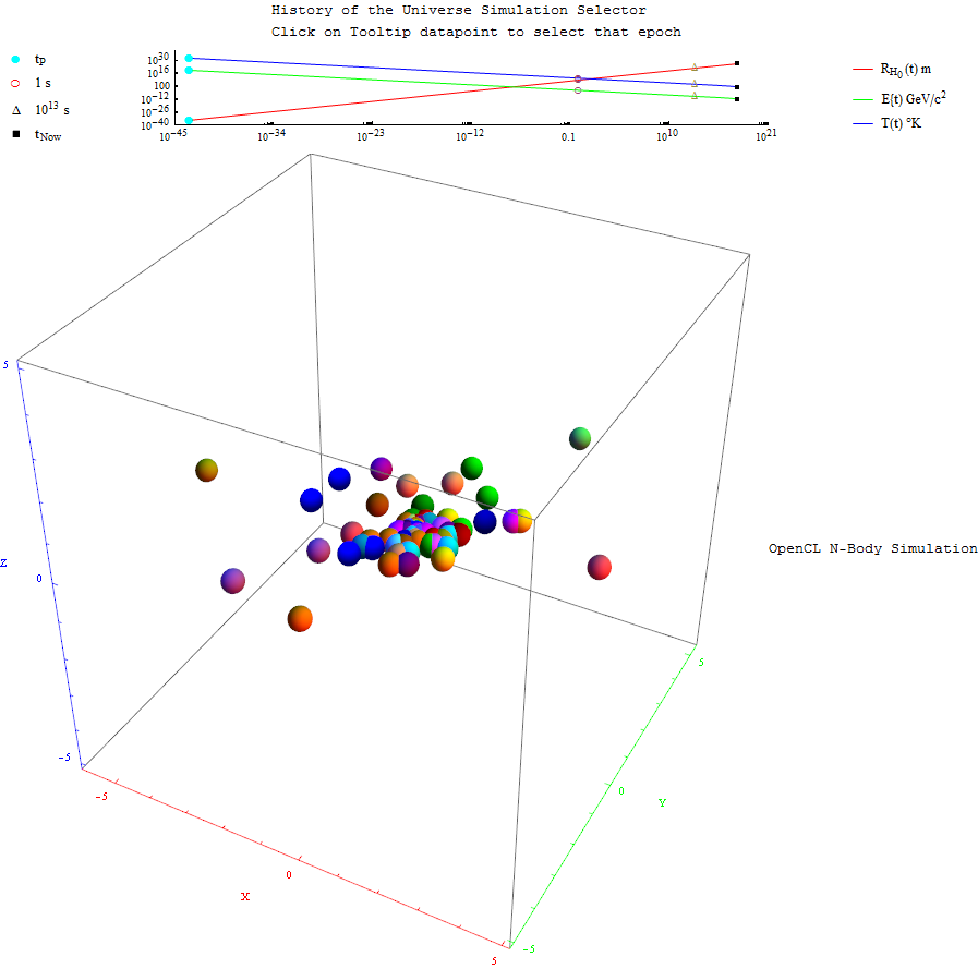
Some visualizations of this in 8D:
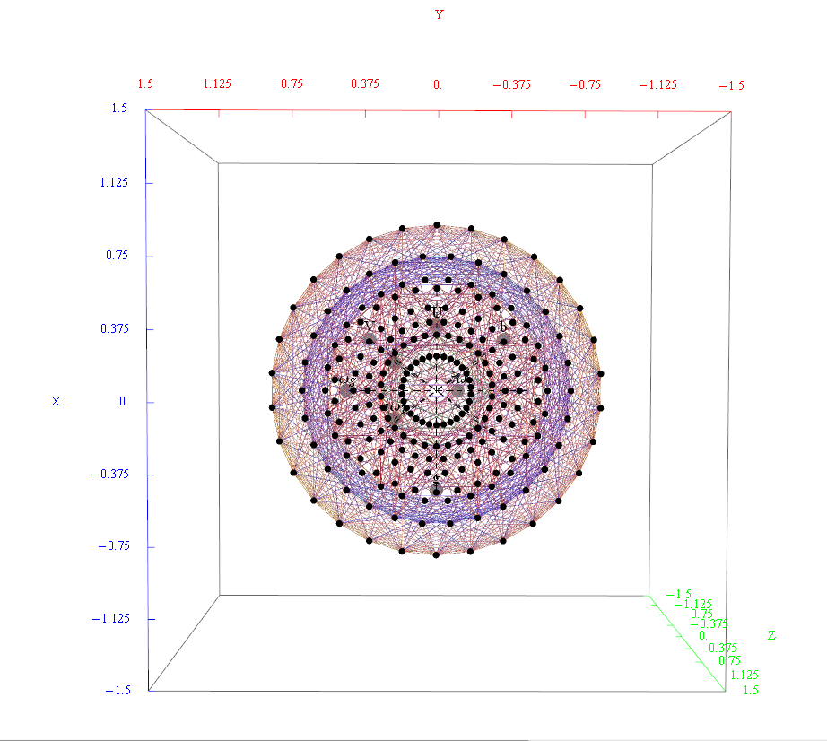
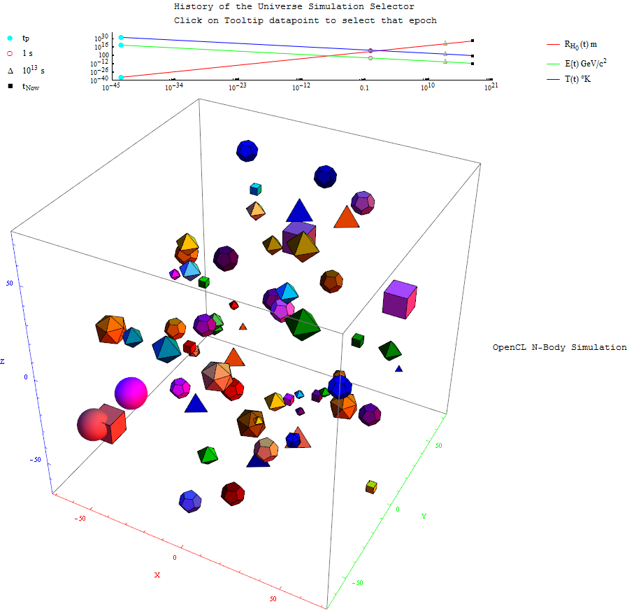
E8-8D-Polytopes-2

to 4D:
E8-4D-Polychora-2

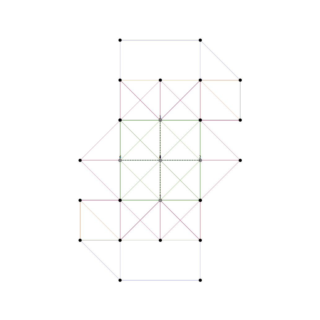
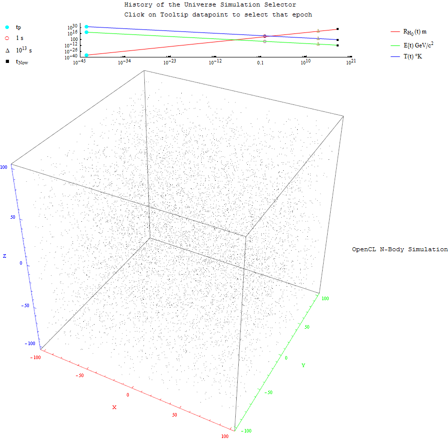
and also showing the Rhombic Triacontrahedron folding from 6D:
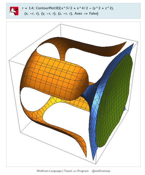
E8-6D-StarPolytopes-2

to 3D:
E8-3D-Platonic-2

Another look at integrating the Pascal Triangle to Clifford Algebra, E8 Lie Algebra/Groups, Octonions and Particle Physics Standard Model

Pascal-g

Modified Lisi split real even E8 particle assignment quantum bit patterns:

Lisi_Particle_Assignments

Assigning a specific mass, length, time, and charge metrics based on new dimensional relationships and the Planck constant (which defines Higgs mass).

ToEsummary

The split real even E8 group used has been determined from this simple root matrix (which gives the Cartan matrix upon dot product with a transpose of itself):

DynkinE8Full.svg

This Dynkin diagram builds the Cartan matrix and determines the root/weight/height with corresponding Hasse diagrams.

E8Hasse

E8HassePoset.svg

Hyperbolic Dynkin Diagrams

I am pleased to announce the availability of the comprehensive set of 238 Hyperbolic Dynkin diagrams ranks 3 to 10. These are enumerated here. They are constructed interactively using the mouse GUI (or manually through keyboard entry of the node / line tables) from this Mathematica notebook or free CDF player demonstration document or interactive CDF player web page.

All of these demonstrations have now been updated to include the new options on Dynkin diagram creation, including left (vs. right) affine topology recognition, black&white vs. color nodes and edges, and for those with full Mathematica licenses the notebook allows for added Dynkin line types.

The Lie group names are calculated based on the Dynkin topology. The geometric permutation names are calculated (to rank 8) based on the binary pattern of empty and filled nodes. The node and line colors can be used as indicators in Coxeter projections and/or Hasse diagrams.

Rank3CompactHyperbolicDynkins1-31bw.svg

Rank3NonCompactHyperbolicDynkins32-75bw.svg

Rank3NonCompactHyperbolicDynkins76-123bw.svg

Rank4HyperbolicDynkins124-176bw.svg

Rank5HyperbolicDynkins177-198bw.svg

Rank6HyperbolicDynkins199-205bw.svg

Rank6HyperbolicDynkins206-212bw.svg

Rank6HyperbolicDynkins213-220bw.svg

Rank7HyperbolicDynkins221-224bw.svg

Rank8HyperbolicDynkins225-229bw_svg

Rank9HyperbolicDynkins230-234bw_svg

Rank10HyperbolicDynkins235-238bw.svg