If anyone is using the E8 to H4 folding matrix in their research, this post provides a bit of context from the original form (2012-2014) as it was improved to the current form. Drop me an email if you are using my work or have questions, or find errors, etc.
See here (Baez), here (Castro-Perelman), and here (Schmidt) for properly cited examples. Of course, many authors may or may not be aware of their use of my prior art without citation (e.g. here (Neilsen) using the fine structure constant α-n as a hyper-dimensional geometric nD scaling factor for the fundamental constants, such as my definition of a new Unit of Measure (UoM) distinct from Natural Units from 1998-2001).
The image below is also available as a Mathematica notebook (NB) or PDF. Click the PNG image for the SVG version.
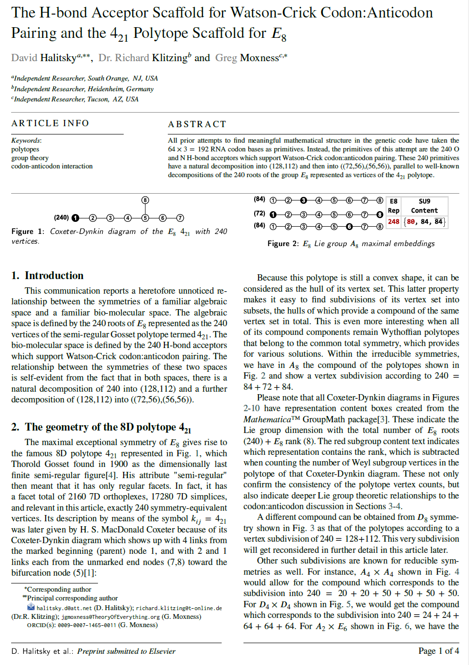
My latest ToE paper here. This paper presents compelling E8 group-theoretic properties that are found in the set of 240 O and N H-bond acceptors which support Watson-Crick codon:anticodon pairing. Empirically correct consequences are deduced from the group-theoretic model.
This paper is related to another recent post here.
Canonical Watson-Crick RNA Codon Acceptor Sites
Here is the WikiMedia version of the Canonical Watson-Crick Acceptor Sites (Figure 11).
This post will document some work I am doing related to E8, H4, and the hypercomplex forms of algebras and groups. So stay tuned….
Hypercomplex numbers
Trigintaduonions derived using repeated Cayley-Dickson doubling of my “Palindromic Octonions” (one of 480 possible) that creates a unique Derivation chart (as shown below). Red are the Octonion triads and Blue are Sedenions.
Sexagintaquatronions derived using repeated Cayley-Dickson doubling of my “Palindromic Octonions” (one of 480 possible) that creates a unique Derivation chart (as shown below). Red are the Octonion triads, Blue are Sedenion, and Green are Trigintaduonions.
Palindromic Octonions (with 7 split forms) and their Cayley-Dickson generated Sedenions with uniquely symmetric Derivation chart and 84 Zero Divisors
This post is a work in process, so check back for the latest visualizations and data. Today (Dec. 31 2025) I finally finished a major update to the section SVG files from the first update of 12/16/2025. Have a blessed New Year for 2026 and beyond!
These were improved a bit on 01/04/2026 and on 01/06/2026 I added more informative Thumbnail icons in the matrix links that include the vertex-edge-face-cell OverallHull images. On 01/12/2026 I added the Snub 24-cell orientations. On 01/20/2026 I improved the visualizations. On 01/26/2026 I increased the thumbnail font and corrected a 24-cell Wythoffian permutation definition.
So if you downloaded previous files, you may want to take another look, as some of the output had anomalous data that didn’t render, along with other errors (due to the way I computed approximate equality between norms). In order to get this done, I realized I was thrashing my Solid State Drive (SSD) due to memory swapping. It died due to that (SSDs have limited writes!), so I had to rebuild the machine with 64 Gb RAM to keep the computations in RAM.
Drop me an email if you find anything that needs correction.
Combined and overall Hulls of Cell-vertex-edge-face first orientations of the OmniTruncated 600 cell (same as 120-cell by Coxeter-Dynkin diagram symmetry). Click the image for SVG version.
For fully interactive Mathematica NB (and higher quality SVG, PDF, as well as PNG files for all of the combined and overall hull pairs as shown above) in all 15 Weyl orbit permutations, download them here:
An example section visualization – the cell-first-cell600-BiRectified-Sections (click to open the SVG version)
Please see several prior posts presenting (with now much improved) sectioning visualizations of Coxeter’s Regular Polytope book Table V here, 120-diminished rectified 120-cell (aka. Swirl-Prism) here, and 90=6×15 matrices of links to the 15 Weyl orbit permutations (with associated Coxeter-Dynkin diagrams) of the 4-polytope 5, 16/8, 24, 600/120 cell sections/animations here.
This post now presents the 60=[4 cell-first, vertex-first, face-first, and edge-first orientations of 15 Weyl orbits] visualizations for the self-dual 24-cell (D4), the disphenoidal 288-cell (F4), and H4 600-cell (which has the same content as its dual the 120-cell by the symmetry of the Coxeter-Dynkin diagram).
These are generated using 4 quaternionic rotations. The one off a main orbit orientation (i.e. using the e0=1 identity quaternion rotation) is either the vertex or cell first orientation for each of the 15 Weyl orbit permutations, with the other rotation being e2+e3. Then for edge and face first orientation rotations, depending on the 24, 288, or 600 cell type, they will be one of either e1+e2+e3 & e1+2e2+e3 (for 24 & 288 cells) or e0+φe1 & e0+e1+e2 (for 600/120 cells).
vZome has a very nice (and fun) website curated by Scott Vorthmann with some information on quaternion generation of cell-vertex-face-edge first orientations here.
The main orbits are (or can also be) generated by using quaternions and the A, B-C, D-F, E-H group theoretic relationships. I actually use octonionic multiplication operations with multiplication tables from the 480 possible where the first (of 7 triads) are the quaternion of 0123. This means the last four dimensions of the octonion (i.e. 4567 or {l, li, lj, lk}) are {0,0,0,0}.
You can navigate the matrices of links below or simply download the ZIP files for the SVG sectioning for the 600-cell here (900 Mb), 288-cell here (200 Mb), and 24-cell here (150 Mb).
SVG section visualizations:
Orientations for H4 600-cell SVG section file links:
Cell Vertex Edge Face
Orientations for F4 Disphenoidal 288-cell SVG section file links:
Cell Vertex Edge Face
Orientations for D4 24-cell SVG section file links:
Cell Vertex Edge Face
MP3 section animations:
Orientations for H4 600-cell MP3 section animation file links:
Cell Vertex Edge Face
Orientations for F4 Disphenoidal 288-cell MP3 section animation file links:
Cell Vertex Edge Face
Orientations for D4 24-cell MP3 section animation file links:
Cell Vertex Edge Face
An interesting set of prisms are in the F4 disphenoidal 288-cell’s omni-truncated sections (below):
An example section visualization – the edge-first-cell288-OmniTruncated-Sections (click to open the SVG version)
If you have access to Wolfram’s Mathematica, see my notebook with code and data that may be helpful here (135Mb). A PDF is here (65Mb). This has detail on the octonion (E82 and E83) based constructions for both the 24D Leech lattices as well as the 16D Barnes-Wall lattice shown at the bottom of this post.
The Leech lattice is a sub-quotient of the largest of the sporadic finite simple groups, namely the Monster group. It is related to (and can be constructed by) E8 and the 23rd Niemeier lattice of E83. The 24D Leech lattice is interesting to the physics of sphere packing, error-correcting codes, and possibly unifying General Relativity (GR) with Quantum Mechanics (QM). String theory was founded on the ideas related to its relationship to the Monster group and how 24 dimensions relate to the bosonic energy levels of the partition function on a torus. For more on the Monster and Group Theory, see my post here.
But taking things down a 8D (Bott periodic) notch, roughly speaking the 16D Barnes-Wall lattice is related to E8 in the same way by BW16=E82.
4320 shortest vectors of BW16using orthogonal projection mapping ℝ¹⁶ → ℝ² (i.e. to B16 basis vectors)
As above with 604800 edges of 16D norm=4 with colors assigned by projected edge lengths
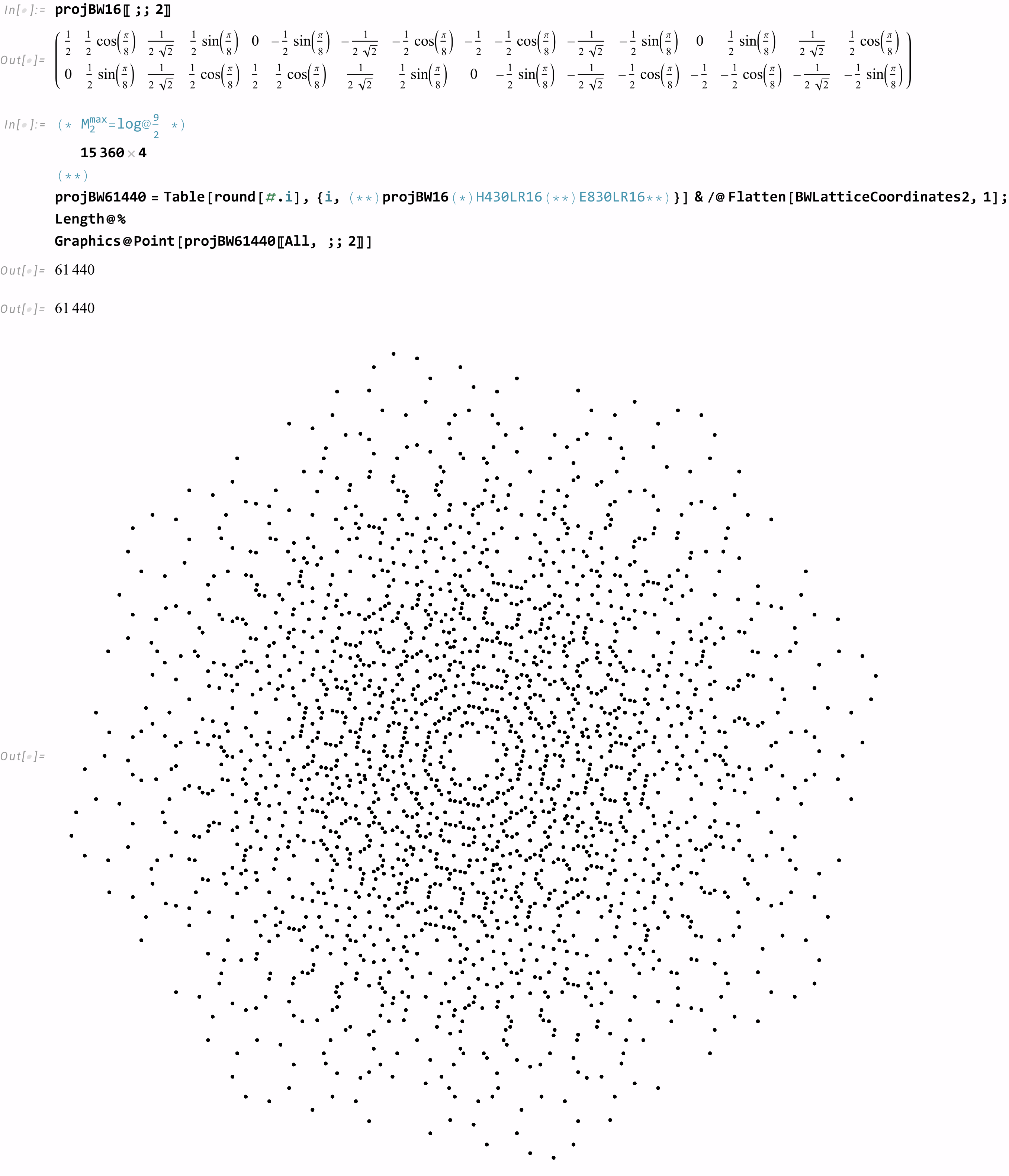
61440 2nd shortest 16D vectors of BW16 using orthogonal projection mapping ℝ¹⁶ → ℝ² (i.e. to B16 basis vectors)
It is interesting to note that if one projects the 61440 2nd shortest 16D vectors of BW16 using orthogonal projection mapping ℝ¹⁶ → ℝ² (i.e. to B8 basis vectors [x=Cos, y=Sin]@(0-15)π/8 used for E8 below vs. the proper (0-15)π/16B16 as done above), we get a similar result as projecting the 2nd shortest 8D vectors of E8 using the same basis shown as grey vertices in Fig 2 of arXiv:2506.11725:
61440 2nd shortest 16D vectors of BW16 projected using the B8 basis vectors. This looks to be the same result as Fig. 2 of arXiv:2506.11725 with grey vertices of the 2160 2nd shortest 8D E8 vertices associated with the maximal magic states in the same projection.
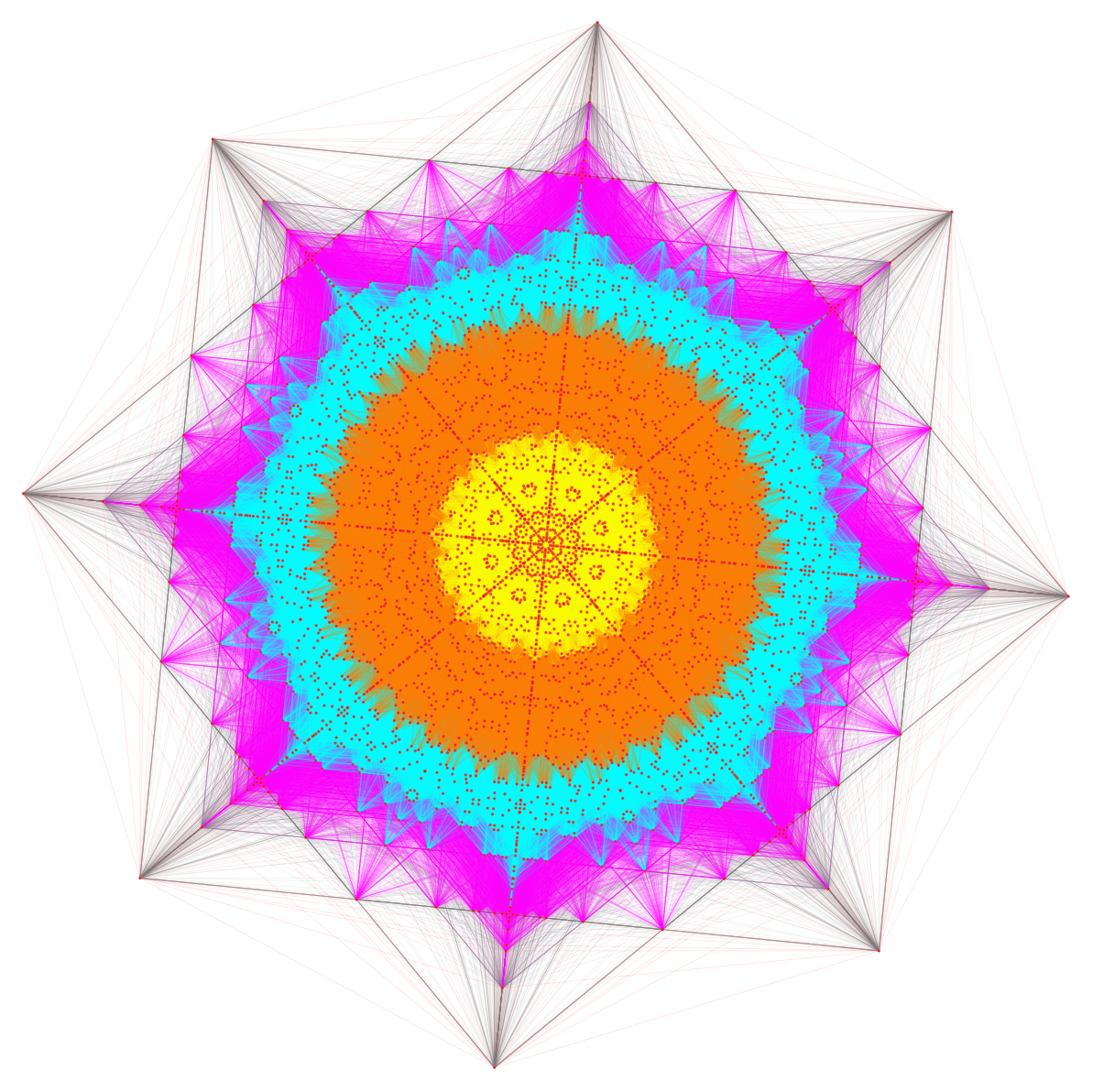
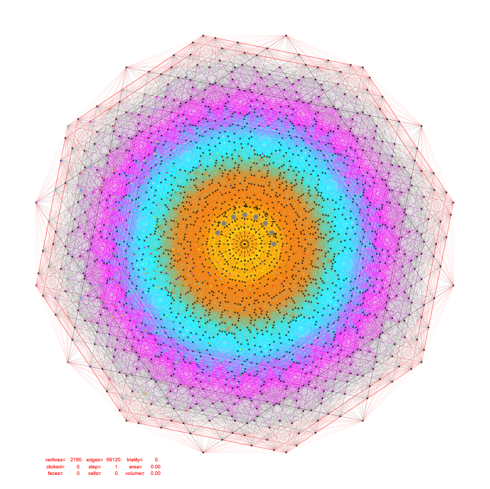
Projecting the 2160 2nd shortest 8D vectors of E8 using the B8 basis vectors including 69120 edges of 8D norm=√8 with colors assigned by projected edge length (notice the similarity in the vertex locations of the figure above):
Projecting the 2160 2nd shortest 8D vectors of E8 using the B8 basis vectors including 69120 edges of 8D norm=√8 with colors assigned by projected edge lengths
Projecting the 4320 shortest 16D vectors of BW16 using orthogonal projection mapping ℝ¹⁶ → ℝ² using the B8 basis vectors [x=Cos, y=Sin]@(0-15)π/8 gives the results shown in Fig. 2 as red and blue vertices:
Projecting the 4320 shortest 16D vectors of BW16 using orthogonal projection mapping ℝ¹⁶ → ℝ² using the B8 basis vectors (0-15)π/8
This time with edges colored by projected edge lengths:
Same as above with 604800 edges of norm=4 with colors assigned by projected edge lengths
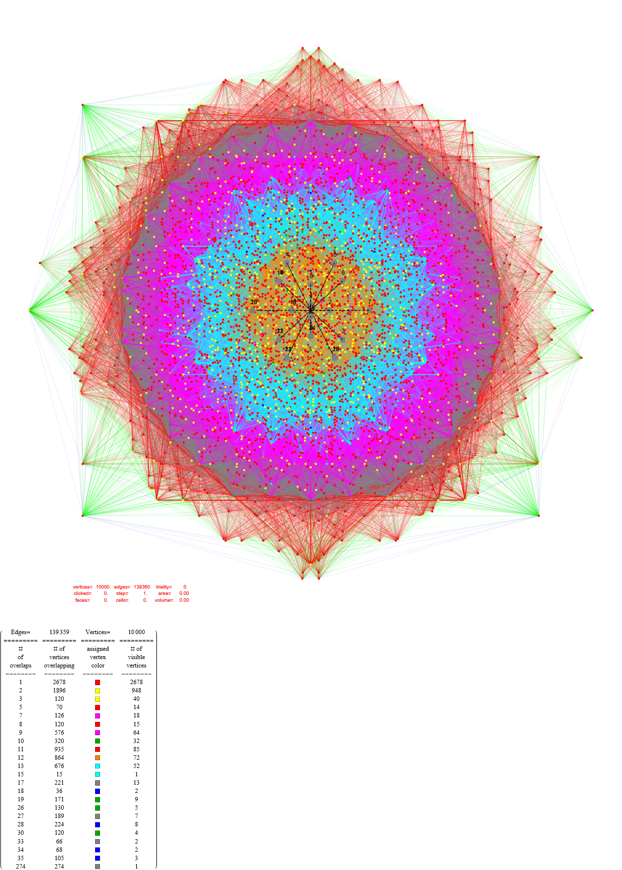
Now, getting creative with the 16D projections of the 4230 BW16, if we double the E8 Petrie basis vectors we get a similar result with 480+1 visible vertices with one at the origin w/240 overlapping vertices. There are 240 yellow with no overlaps and 240 blue with 16 overlaps each. There are 604800 norm=4 edges using roughly the same color pallet as my WP E8 Petrie image. This makes it easier to see the difference between the 4230 BW16 and the normal E8 Petrie projection, which seem to share the grid-like pattern of the 24-cells within the folded E8 = H4 + φ H4 :
16D projection of the 4230 BW16 using the E8 Petrie basis vectors doubled
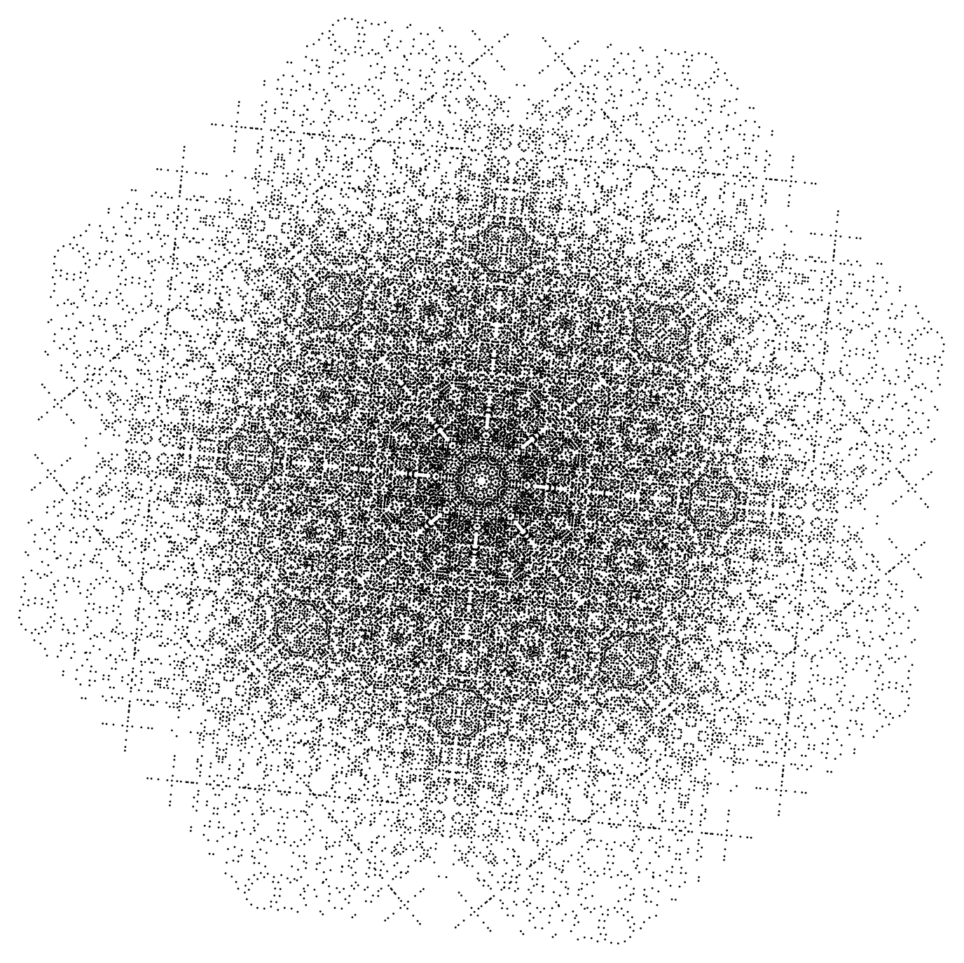
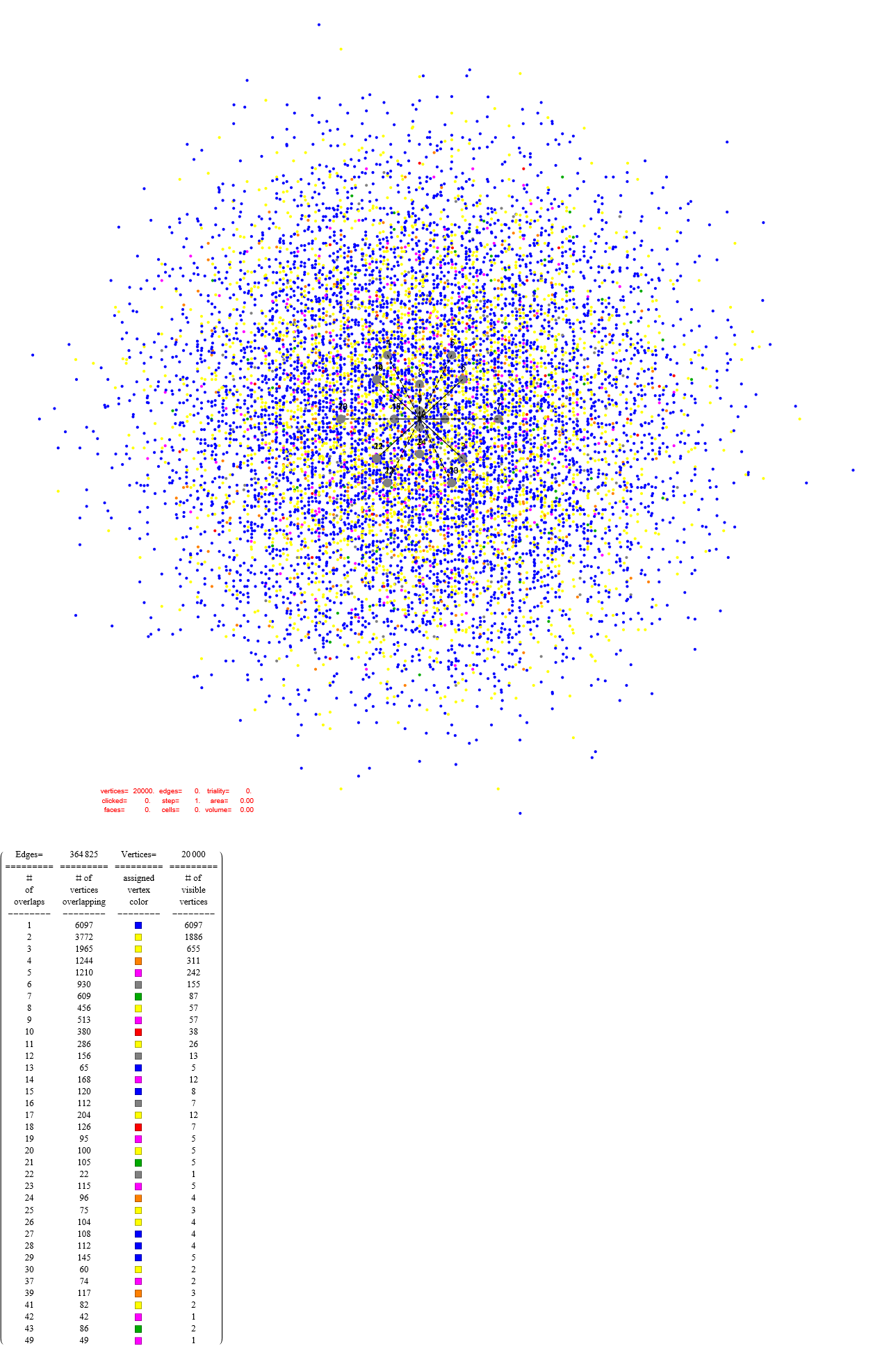
This is the same as above, but using the 61440 vertex BW16 with no edges (given there are millions of them). Please note that the number of visible vertices is the same as E8241 at 2160!
16D projection of the 61440 BW16 using the E8 Petrie basis vectors doubled with 2160 visible vertices
Octonion based Barnes-Wall and Leech Lattice visualizations based on my implementation of work from Geoffrey Dixon and Robert Wilson:
Octonion defined Barnes-Wall to 16D B82 projection
Octonion defined 24D Leech lattice to 8D E8 Petrie projection with all 196560 vertices in 2D and 3D, noting the similarity to the 6720 vertex rectified E8 in the same projection (above).
Octonion defined Leech lattice to 24D E83 Petrie projection with 20 increments of 1000 vertices for every 10000 out of 196560
Same as above with 50% of the inner edges filtered out
Video(s) of 4D geometry in “3D Flatlander views” (i.e. what it looks like if objects from 4 “other” dimensions pass through an area of our 3D world for a period of time (i.e. 34 s)
This page presents the comprehensive 15 permutations of the six 4D polychora (i.e. 5, 16/8, 24, 600/120 cells) in full SVG format for convenient use in high quality academic papers on the topic (e.g. simply save the SVG and edit in Inkscape or other tool to produce PDF or PNG, etc.). You are free to use these under Creative Commons Attribution-ShareAlike 4.0 International CC BY-SA 4.0 with appropriate attribution. Drop me an email if you find anything that needs correction.
My cell-first and vertex-first {5,3,3} 120-cell section visualizations with subgroup sections (when the inscribed solid has more than one permutation in its orbit) are available in Wikipedia Commons here and here. Let me know if you need customized hyper-complex and/or hyper-dimensional group-theoretic projection/section visualizations, as my extensive Mathematica code-base may be able to generate it.
The content below uses a 6×15 matrix of 4D to 3D projections of the convex hulls, each with a link to a page with that objects Coxeter section decomposition. I want to give a shout-out (cite) qfbox.info and polytope.miraheze.org for providing vertex coordinates used in the creation of the objects. The Vertex-Edge-Face-Cell first sections are in another one of my posts here.
There is also another 6×15 table with links to video animations of the sections in the 4D to 3D flatlander from Left/Right (or minus to plus). This is an analog of 3D objects passing through the 2D planar world of flatlanders.
Also available is a Mathematica notebook (360Mb) with code to produce the 4D vertex data as well as the visualized interactive 3D objects. See also an overview of these lists explained in a this Powerpoint presentation, which covers the isomorphisms between them due to the symmetries in the A4, BC4, and H4 Coxeter-Dynkin diagrams that represent them.
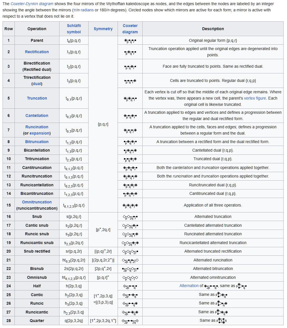
Below are some screenshots from a PPT I created to explain the organization. Some of this content is now on Wikipedia from my updates to those pages. The PPT is available here (in PDF here) or you can click on the PNG images (below) to get the SVG versions:
Wythoffian 4-polytope operation table with row index to the D4 chart above. Please not, this chart is based on the BC4 Coxeter-Dynkin diagrams of the 16-cell / 8-cell (tesseract), not the D4 equivalences.
Comparing the D4 Coxeter-Dynkin diagram operations with triality equivalence to the B4/C4 24-cell=16-cell+8-cell
I took screenshots of a few qfbox.info pages to annotate the differences in layout below. Please note the palindromic binary Weyl group orbits and operation equivalences between them:
Comparing the 24-cell polytope operations ordering: Note the palindromic binary Weyl group orbits
Comparing the 16-cell / 8-cell polytope operations ordering
The Coxeter-Dynkin diagram relationships between the BC4, D4, and F4 are as follows (my apologies to those who might be irritated by my use of filled nodes instead of the “ringed” nodes):
The 600-cell (parent H4) + φH4 are 4 dimensions of a rotated (folded) 8D E8 4_21 polytope with 240 vertices and 6720 edges (just as D6 folding gives the H3 parent)
Links to the SVG Section Files:
A4
BC4
BC4
D4’+ D4 =F4
H4
H4
5-cell
(16-cell
+ 8-cell
=24-cell) (24-cell+ Dual24cell =288-cell)
600-cell
120-cell
Links to Sectioning MP4 Video Animations (i.e. 4D to 3D Flatlander):
A4
BC4
BC4
D4’+ D4 =F4
H4
H4
5-cell
(16-cell
+ 8-cell
=24-cell) (24-cell+ Dual24cell =288-cell)
600-cell
120-cell
For completeness, I am also including a table of 3D polyhedra, namely the Platonic, Archimedean, and Catalan Solids including their irregular and chiral forms. These were created using quaternion Weyl orbits directly from the A3, B3, and H3 group symmetries
.
Platonic, Archimedean, and Catalan Solids
Another post with more detail on the 5-cell (A4) SU(5)->SU(4) maximal subgroup content generated via quaternions is here.
This is an analysis of the Coxeter Sections for the Swirl Prism 120-Diminished Rectified 600-Cell. The source data, which can be found on either of two polychora sites (qfbox.info and polytope.miraheze.org) seems to have two missing vertices 598 as generated by their permutation lists (vs. the intended 600). The data below, with an added two vertices of {-1,-1,φ3, φ3} and {1,-1,φ3, φ3} in the suspected error sections #3 & #15, is shown in data and 3D convex hull and Coxeter sectioning forms.
Video(s) of 4D geometry in “3D Flatlander views” (i.e. what it looks like if objects from 4 “other” dimensions pass through an area of our 3D world for a period of time
The 3D XYZ convex hull projections (with W=0) on the right and the +/- W Coxeter Sections of the (vertex-first) rectified 600-Cell with 720 vertices on the left with framed center as subsections of sections.
The XYZ 3D convex hull projections on the right and Coxeter Sections of the Swirl Prism 120-diminished rectified 600-Cell with 600 vertices on the left with framed center as subsections of sections.
The Coxeter Sections for the 120 diminished vertices (i.e. the complement of the Intersection of the (vertex-first) Rectified 600-cell and the Swirl 120-Diminished Rectified 600-Cell)
List of vertices for the Rectified 600-cell
List of vertices for the Complement of the Intersection of the Rectified 600-cell and the Swirl 120-Diminished Rectified 600-Cell
The palindromic E8, Space-Time Algebra (STA Hodge star) octonion/biquaternions, and the RNA [CU;AG] codon genome genomatrix can be integrated into a possible isomorphism between an E8 (or one of its maximal subgroups) based Theory of Everything (ToE i.e. unifying a 3 generation Grand Unified Theory (GUT) of the Standard Model (SM) with General Relativity (GR)) and the biochemistry of Life itself. It does this from a single mathematical 240+8 dimensional exceptional Lie algebra, group (and subgroups), lattice (and codes), and associated nD polytopes in a Grand Objective Design trinity with triality based triads.
The compendium of 8×8 matrices (below) use the RNA [CU;AG] proteins (Cytosine, Uracil, Adenine, Guanine) vs. the DNA [CT;AG] where Thymine replaces Uracil.
The palindromic isomorphism of E8, STA Hodge star octonion/biquaternions, and the [CU;AG] codon genome genomatrix
It is a matrix integration of my E8-H4 Folding (Rotation) matrices, the STA Hodge star octonion/biquaternion multiplication matrices, and the [CU;AG] Codon genome genomatrix. The genomatrix is a modified form of that presented by Sergey V. Petoukhov, Head of Laboratory of Biomechanical System, Mechanical Engineering Research Institute of the Russian Academy of Sciences, Moscow in a 2011 paper arXiv:1102.3596 “The genetic code, 8-dimensional hypercomplex numbers and dyadic shifts”.
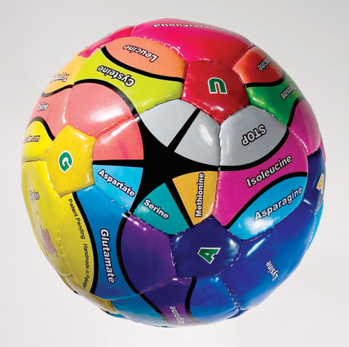
The linkage between the genomatrix and E8 is not surprising when understood in the light of how E8 folds to 4 copies of the H4 4D duals of the 600/120-cells, which have the convex hull of the chamfered dodecahedron. This 3D shape is similar to the truncated icosahedron (aka. soccer ball) used in the (2003 abandoned patent) mnemonic created by Mark White and documented in 2007 arXiv here “The G-Ball, a New Icon for Codon Symmetry and the Genetic Code”. There is an interesting blog post in American Scientist about that here.
Truncated Icosahedron (aka. soccer ball) Codon by Mark White (image linked from Bryan Hayes “Ode to the Code”).
The H4 Cell-First {5,3,3} 120-cell (J), dual of the 600-cell, showing the hull of the chamfered dodecahedron. It is also called a truncated rhombic triacontahedron. It can more accurately be called an order-5 truncated rhombic triacontahedron because only the order-5 vertices are truncated. It is shown with physics particle assignments.
The H4 Cell-First {5,3,3} 120-cell (J) with physics particle assignments
The H4 Vertex-First {5,3,3} 120-cell (J’) with physics particle assignments
The germ of this idea (pardon the pun) seems to have come from Petoukhov in 1981 (as per his list of works here) in a paper “Investigations on Non-Euclidean biomechanics. Projective geometry, Fibonacci numbers and the kinematic scheme of human body.” He seems to have used Manfred Eigen’s work beginning in 1971 with “Self-organization of matter and the evolution of biological macromolecules”.
These ideas were improved on by David Halitsky in 1993 in “A geometric model for codon recognition logic”. I also credit the late Frank Dodd Tony Smith Jr for highlighting this in his personal research ideas (along with many other interesting ideas to E8 and Cl(16) based objects). This was done here.
It is interesting to note that the particular octonion (or Hodge Star BiQuaternion) multiplication matrix used by Petoukhov is the same one as highlighted in my recent papers and blog posts regarding the most beautiful of the 480 octonion symmetry pattern, which I introduced in my “Isomorphism of H4 and E8” arXiv paper here and discussed in a bit more detail here “Space-Time-Algebra (STA) Octonionic Illustration”, with this summary:
"This was originally introduced in my (always updated/corrected) last few papers here and here (or if you prefer to get the originals off arXiv here and here). It happens to be the first canonical triad (with Fano plane index fPi=1) with 16 sign-mask set of sm=5 taking the first sign-mask in that set being hex 08H (which reverses triad 4 from 246→264). This not only naturally produces a palindromic RCHO Standard model with E8 vertex counts, the STA Hodge star elements are in the reverse diagonal made up of e7's, its non-null Derivation has en with n= {1,2,3,4,5,6,7} with the unique split derivations being the 7 triads in order. It is the only octonion of the 480 that has that property! There are only 6 others (out of 48 total starting with the canonical quaternion first triad of {1,2,3}) that have the triad derivations, but the triad node orders are mixed along with the multiplication table +/- signs in the last row being mixed across {0,1,2,3} and {4,5,6,7}."
8×8 E8 and Octonion Matrices
E8 with physics particle assignments shown in triality based triad projection (blue edges show particle generation and/or color trialities)
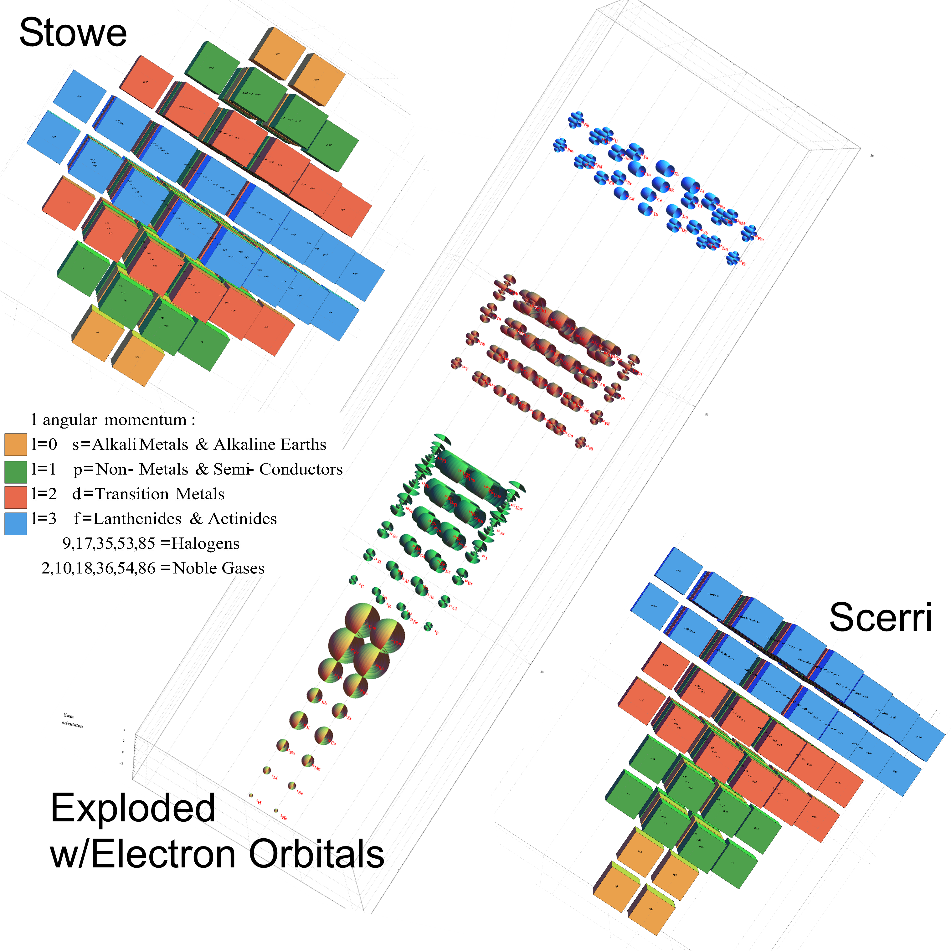
For completeness, we show below the palindromic 4D (3D+Color) projection of the Atomic Element Periodic Table of Quantum Chemistry below:
3D/4D Octahedral/4-Orthoplex projection (Stowe) of a 4D Periodic Table with angular momentum color coding and spherical harmonic element orbitals. Note: the palindromic structure of 8 groups of 120 elements isomorphic to the 120 vertices of the H4 {5,3,3} 600-cell (then include anti-atoms for 240 total elements).
2D Periodic Table with angular momentum color coding and spherical harmonic element orbitals. Note: the palindromic structure of 8 groups of 120 elements isomorphic to the 120 vertices of the H4 {5,3,3} 600-cell.
In a post from 2013, I summarized the findings of my original 1997 paper (updated in 2007) documenting a new FineStructureConstant (α) based set of definitions for the fundamental constants (c, ħ, GN, and H0) . That post was needed due to updates from 2013 Planck spacecraft CMB (H0) results and the 2012 LHC confirmation of finding the mass of the Higgs boson (mHiggs).
It is interesting to note that the added factor of λcnv over H0, which is based on the Compton wavelength of the electron/proton mass ratio (as is gc), precisely accommodates the Hubble tension!
About the same time, Wolfram Mathematica deprecated their PhysicalConstants package in order to provide for more robust curated datasets (e.g. CODATA ParticleData) which includes Quantity (exact or with experimental uncertainties) and UnitConvert capability.
I had maintained my own version of this package in order to add a custom UoM with conversions between it and the SI UoM based on my analysis of a possible unification of the fundamental constants and dimensional relationships of (L)ength, (T)ime, (M)ass, and (C)harge. These strongly indicate an 8D (E8) fine structure linked a posteriori particle mass prediction of the Higgs boson mass=124.44 GeV/C2 and cosmological constants of gravity (GN) and H0.
This post provides for the integration of that newer Wolfram Mathematica capability as well as the 2019 redefinition of the SI UoM which replaced some measures with exact unit definitions. These changes are described on Wikipedia here and by Wolfram’s Chief Scientist Michael Trott here.
My Powerpoint overview is here with the first slide shown below:
Mass-Length-Time (MLT) UoM with Fundamental Constants compared with SI UoM with 2019 exact and experimental error bars.
This new Time Unified UoM identifies a UnitLength= α/Rydberg Constant (R∞) associated with atomic mass spectroscopy and UnitAcceleration that is 4π(cH0=Acceleration AssociatedWith CosmologicalExpansion Rate) as a a dimensionless unit with UnitLength=(complexified UnitTime)2. It links the macro (cosmological) to the micro (nuclear/chemical) scales via integer exponents (dimensions) related to the FineStructureConstant (α). Other notable defining constants are a 4D (TimeUnit4) UnitCharge and 8D c=α-8 UnitVelocity, h=α-8 UnitAction, and Newton’s GravitationalConstant (GN~4πH0~α8/UnitTime).
See below a list of the constants and UoM elements for SI, Natural (Planck or geometrized) units, and my own “more Natural” Time Unified UoM, which includes the Higgs mass (a posteriori) postdiction. The list is sorted by n where (Tn) is the unified (reduced) time dimension of the physical constant or UoM.
Mass-Length-Time (MLT) UoM with Fundamental Constants compared with SI UoM with 2019 exact and experimental uncertainties (as well as in comparison to the Natural Planck units recovered by setting α=1).
Mass-Length-Time (MLT) UoM code snippets used to create the above chart.
In a recent Azimuth post, John Baez discussed the McGee group and (3,7)-cage graph. A link to a conversation on MathOverflow describes its connection to the Fano plane and the octonions via the Heawood graph (which he had discussed on his Visual Insight blog here).
So I thought it would be fun to show how the alternate graph of the McGee group shown on WP is indeed the 24-cell with 64 of 96 edges removed being projected to the B4 Coxeter plane. So again, it is linked to E8=H42 (as 4 4D Left (L)/Right (R) golden ratio (φ) scaled 600-cell=24-cell+snub 24-cell from the E8 to H4 rotation or folding matrix). Another related post here shows how the E8 Petrie projection decomposes into the two sets of 4 rings as H4 and H4φ 600-cells.
User:Leshabirukov’s Alternate McGee graph is here and below with blue edges being the 4 dimensional axis:
Below are renderings from my hyperdimensional hypercomplex (quaternion/octonion/sedenion) VisibLie_E8 viewer:
McGee Group (3.,7)-cage graph as a 24-cell projected to the B4 Coxeter plane with 64 edges removed (and including 4 axis “edges” for a total of 24 vertices and 36 edges)
To get a view of how B4 projection is isomorphic to the Greg Egan animation, below is my animation overlaid on top of it:
The animation showing the isomorphism between Egan’s base image and the H4φ 24-cell projected to the B4 Coxeter plane.
The first frame is Greg Egan’s base image in the Baez article. Each frame is 2 seconds.
The second frame adds the XYZW axes annotations (4 pairs of red node links that are antipodal across the labeled axis letter (e.g. the nodes above/below the black X line are connected by Y axis endpoints with p#’s 56 & 201, the nodes above/below the black Y line are connected by X axis endpoints with p#’s 74 & 183). These red endpoints are all associated with the 16-cell (i.e. 4-orthoplex octahedron) within the 24-cell.
The third frame differentiates the the inner(cyan) / outer (purple) octagon rings. These two rings are each 8 of 16 vertices of the 8-cell (i.e. 4-cube Tesseract) within the 24-cell.
The 4th frame adds the vertex numbers (p and p*) split between #=1-128 and 257-# (as respectively palindromic 256-129) which are always antipodal in the X-Y axis of the B4 Coxeter plane projection (or any other Coxeter plane projection) as well as being antipodal within each of the 4 sets of 6 nodes in the Egan animation.
A static image for ease of analysis.
24-cell with all of its 96 edges projected to the B4 Coxeter plane. Vertex numbers are from a canonical sort of E8 in Pascal triangle order (when including the 8 generator and 8 anti-generator vertices as 2-9 and 248-255 (respectively).
For anyone who studies deeply the E8 to H4 connections as I do, you know the L/R H4 and H4φ 24-cells have the same palindromic L/R 4D elements in the E8 vertices as well. This means the E8 based McGee groups overlap identically, as shown here:
H4 and H4φ 24-cells in B4 Coxeter plane projection
So, here is the full E8 in the same Coxeter B4 projection with vertex coloring based on the overlap counts.
How the E8 H4 and H4φ snub 24-cells (as 4 π/5 rotations of each of the φ scaled 24-cells) fill in this E8 projection with more McGee groups is more interesting and complex. The patterns for the removal of the specific edges are also interesting and inform the possible physics of E8 based unification theories.
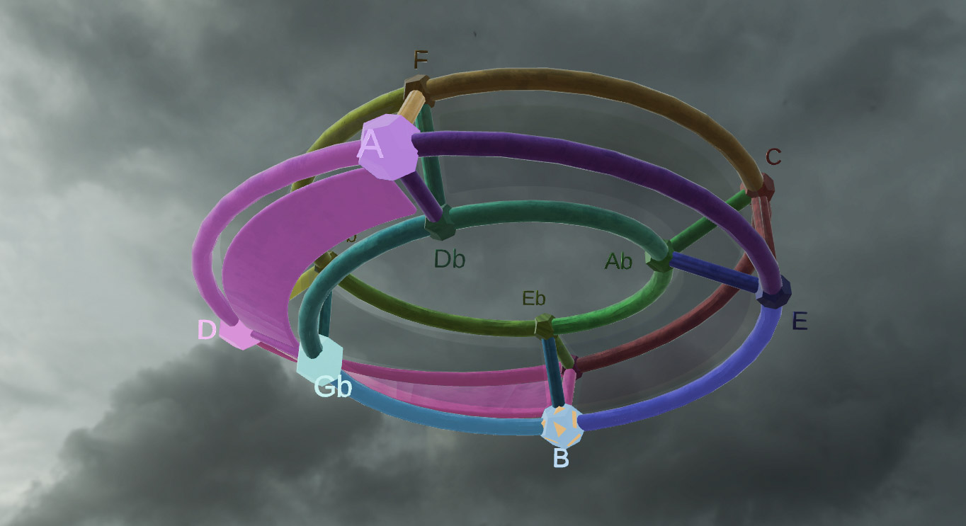
… and a McGee graph torus’ fascinating connection to the world of music….
What the author calls the “Cholidean Harmony Structure”
Picture the same red WXYZ 4D axis node-pairs (not shown in this image) positioned at the centroid of the triads. It has 12 vertices and 24 edges. The full 24-cell McGee vertices has a 4D-hexadic structure with mirrored triadic pairs across edge-connected axis nodes.
Analogously, if we view the McGee torus as 4 rings of 4-edges (plus 4 sets of 4 WXYZ quaternionic axis-connected edges), one could then view musical harmony as being represented with 3 (Complex or Imaginary) rings of 4 edges each forming the triads (and excluding the Real component and its axis connections).
This difference might be understood by looking at the composition of the hyperdimensional hypercomplex functions (e.g. quaternion / octonion Exp / Cos / Sin / Octonionic Fourier Transform (OFT) ) with respect to Im vs. Re differences.
Dedicated to the pursuit of beauty and Truth in Nature!


