
Images
Interactive Reimann Zeta Function Zeros Demonstration
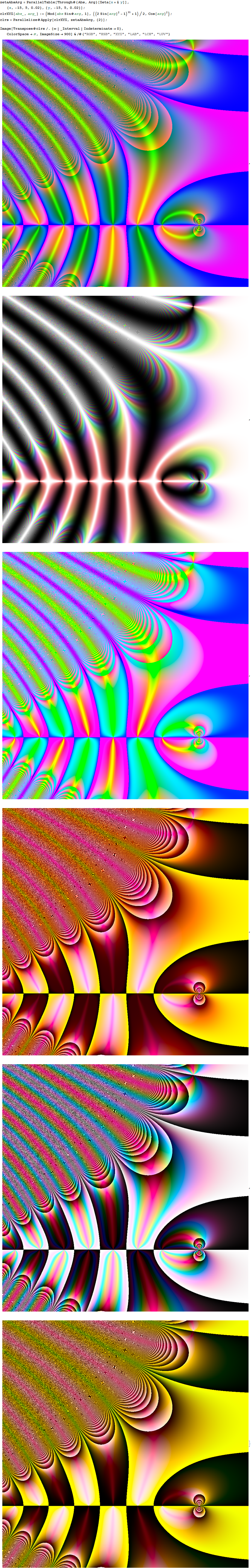
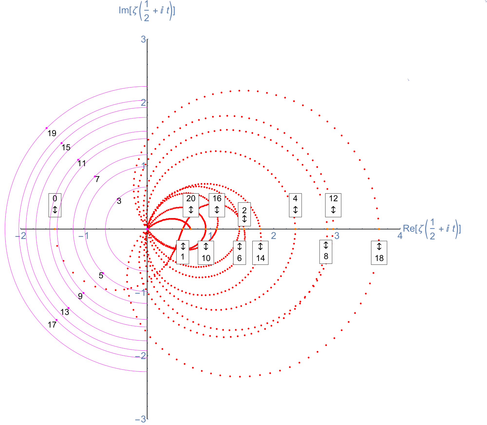
This web enabled demonstration shows a polar plot of the first 20 non-trivial Riemann zeta function zeros (including Gram points) along the critical line Zeta(1/2+it) for real values of t running from 0 to 50. The consecutively labeled zeros have 50 red plot points between each, with zeros identified by concentric magenta rings scaled to show the relative distance between their values of t. Gram’s law states that the curve usually crosses the real axis once between zeros.
A downloadable copy is available ZetaZeros-local-art-50.cdf Latest: 05/23/2016.
Note: The interactive CDF plug-in as required below does not currently work on Chrome browsers.
A Snapshot picture for those w/o Wolfram CDF interactivity:
Selectable example code snippet:
[wlcode]Show[ListPlot[Style[pts2, Red], PlotRange -> {{-2, 4}, {-3, 3}},
AspectRatio -> 1, ImageSize -> imageSize,
AxesStyle ->
Directive[Thick, If[artPrint && ! localize, Large, Medium]],
Graphics[{PointSize@.01,
tttxt := If[artPrint && ! localize, tttxt1, ttxt0];
If[ttxt0 = ToString[# – 1];
Abs@zeroY[[#, 1]] < 10 chop,
(* Magenta Critical Line Zeta Zeros *)
tttxt1 =
Column[{ToString[# - 1], "t=" <> ToString@zeroY[[#, 4]]},
Center];
ttLoc =
zeroY[[#, 4]] If[artPrint && ! localize, 1, 2] imagesize/40000;
(* Flip Point Labels above/below the X axis *)
ttLoc1 = {-1, (-1)^Round[#/2]} ttLoc/Sqrt[2];
{Magenta, Point@ttLoc1,
Circle[zeroY[[#, ;; 2]], ttLoc, {1, 3} \[Pi]/2],
Black,
Tooltip[Text[
Style[tttxt, If[artPrint && ! localize, Large, Medium, Bold]],
(* Shift the Labels off the Point *)
ttLoc1 (1 – (-1)^Round[#/2] .05)], tttxt1]},
(* Orange Critical Line Imaginary zeros w/Real>0 *)
tttxt1 =
Column[{ToString[# – 1], “x=” <> ToString@zeroY[[#, 1]],
“t=” <> ToString@zeroY[[#, 4]]}, Center];
{Tooltip[{Orange, Point@zeroY[[#, ;; 2]], Text[Style[
Column[If[EvenQ[Round[(# – 1)/2]], Prepend,
Append][{“\[UpDownArrow]”}, tttxt], Center,
Frame -> True],
Black, If[artPrint && ! localize, Large, Medium],
Background -> White],
(* Flip Point Labels above/below the X axis *)
zeroY[[#, ;; 2]] + {0, (-1)^Round[(# – 1)/2]} If[
artPrint && ! localize, 1,
If[artPrint, 4/1, 3]] imagesize/5000]},
Column[{ToString[# – 1], “x=” <> ToString@zeroY[[#, 1]],
“t=” <> ToString@zeroY[[#, 4]]}, Center]]}] & /@
Range@Length@zeroY,
Magenta, Disk[{0, 0}, .03]}]][/wlcode]
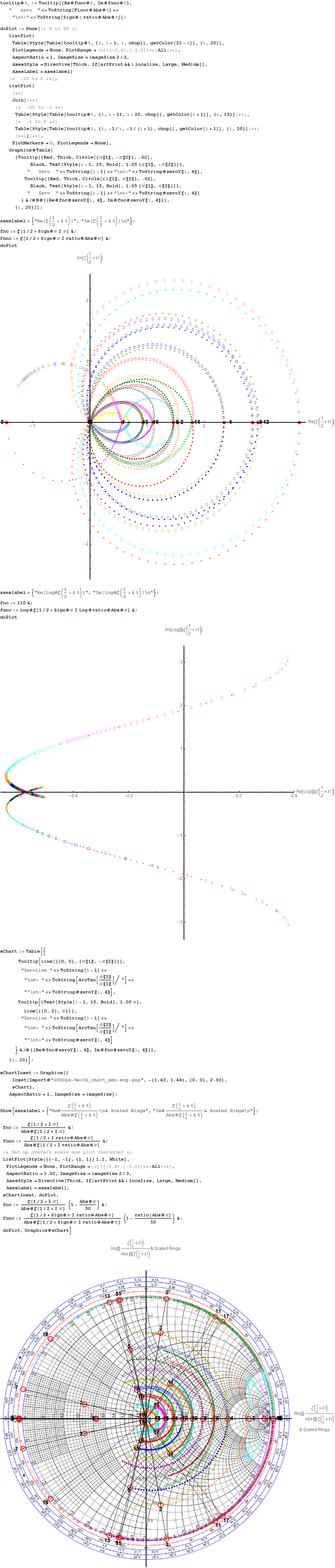
More plots with various scaling functions and multi-color coding along with Tooltip on mouse-over. Bear in mind the last Smith Chart with a division by Abs@Zeta indicates where the increments go exponential near the 0.
A Snapshot picture for those w/o Wolfram CDF interactivity:
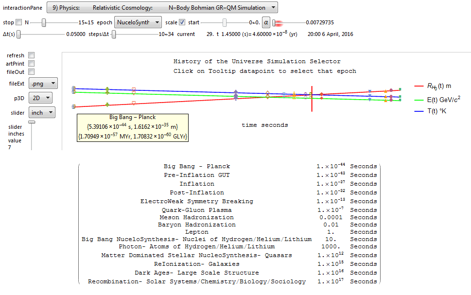
15 Epochs and 60 Orders of Magnitude – History of the Universe
E8 in E6 Petrie Projection
An article (interview) with John Baez used an E8 projection which I introduced to Wikipedia in Feb of 2010 here. Technically, it is E8 projected to the E6 Coxeter plane.
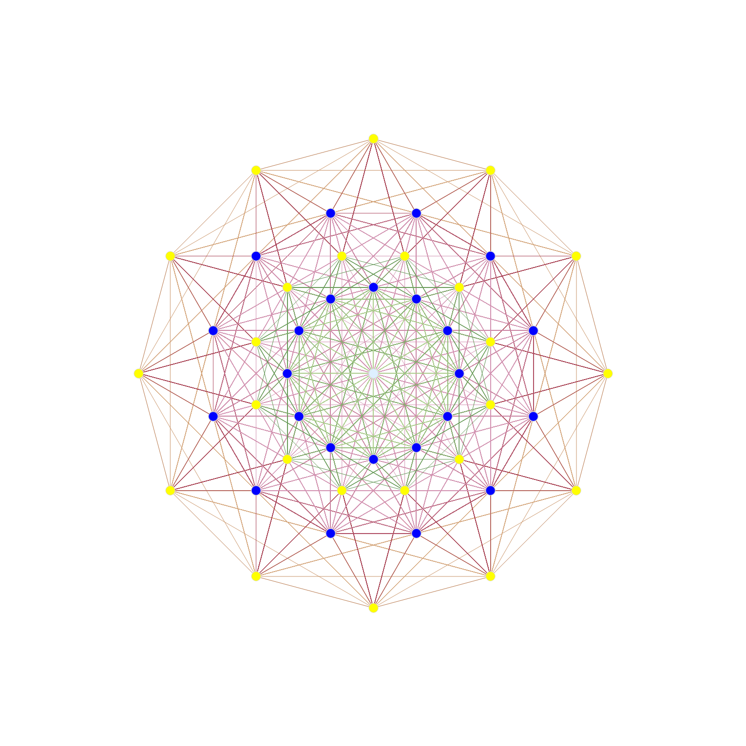
The projection uses X Y basis vectors of:
X = {-Sqrt[3] + 1, 0, 1, 1, 0, 0, 0, 0};
Y = {0, Sqrt[3] – 1, -1, 1, 0, 0, 0, 0};
Resulting in vertex overlaps of:
24 Yellow with 1 overlap
24 Dark Blue each with 8 overlaps (192 vertices)
1 Light Blue with 24 overlaps (24 vertices)
After doing this for a few example symmetries, Tom took my idea of projecting higher dimensional objects to the 2D (and 3D) symmetries of lower dimensional subgroups – and ran with it in 2D – producing a ton of visualizations across WP. 🙂
It was one of those that was subsequently used that article from the 4_21 E8 WP page.
Here is a representation of E6 in the E6 Coxeter plane:
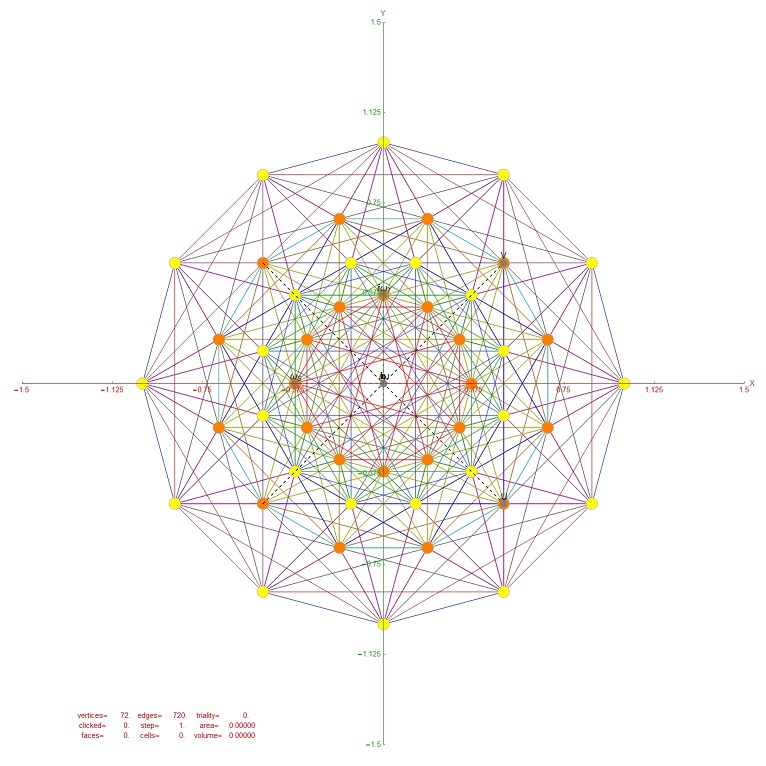
Resulting in vertex overlaps of:
24 Yellow with 1 overlap
24 Orange each with 2 overlaps (48 vertices)
More Fibonacci / Pascal Triangle Patterns
Last year I posted this on Pascal Triangle Modulo 2 thru 9 and their Sierpinski Maps.
I just saw an interesting post by Lucien Khan on some Theological numerology (gematria) as it relates to the Modulo 10 patterns of Fibonacci here.
I verified the pattern and added a few more as it relates to the repeating Modulo 9 and 10 patterns, Pascal Triangle and E8 (as in my original post).
Numbers are highlighted when divisible by:
60 are in red
30 are in green
15 are in blue
12 are in magenta
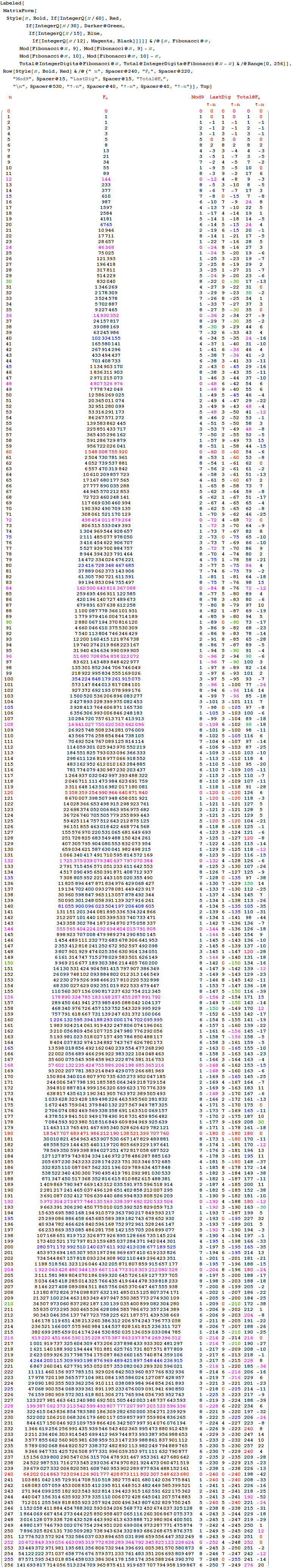
This is all tied to the Pascal Triangle with its 2^n binary (Clifford Algebra) representation, E8 and the number 4!=24 and Octonions.
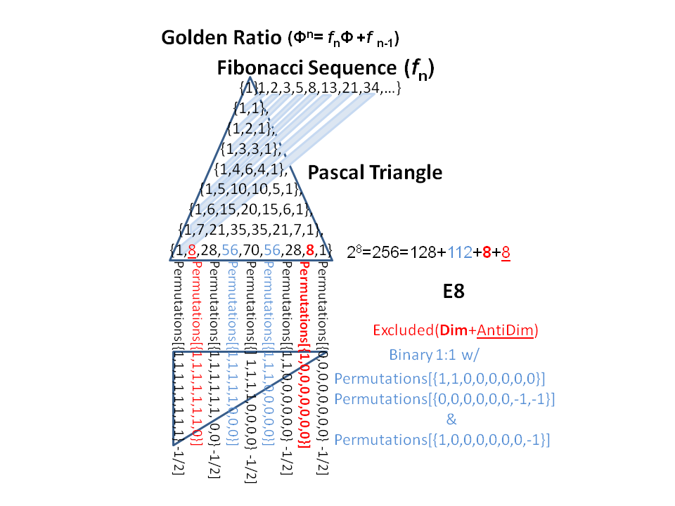
All of these structures, including the 3 dimensional geometry of the Platonic solids (and its big brother, the 4D non-crystallographic H4 group geometry) are related to E8 via a folding matrix I determined a few years ago here.
For some related interesting reading from John Baez regarding the number 24 and its link to String Theory (M-Theory) updated from last week! (see also related info on his other favorite numbers 5 and 8).
Introducing the Sedenion Fano Tesseract Mnemonic
The Sedenion “Fano Tesseract” Mnemonic is an extension of the “Fano Cube” idea introduced by John Baez in his much cited blog post. The Fano Cube identifies each valid each triad by a hyper-plane which intersects the e_0 node.
Notice in this VisibLie_E8 output for the pane #3 “Fano Visualization Demonstration”, there are 35 sedenion triads, 7 of which are from the octonion used as an upper left quadrant base for a Cayley-Dickson doubling (highlighted in red).
The 16 vertices of the tesseract are sorted by the same “triad flattening” process used to construct a consistent Fano Plane Mnemonic for all 480 unique octonion multiplication tables.
As in the Fano Cube, the edges are highlighted in Cyan if they are selected in the n1-n3 buttons. Unlike the Fano Plane and Cube, the edges represented by the split octonion multiplication table columns/rows are not highlighted in red.
While there are 32 edges in the formal tesseract, each valid sedenion triad is identified by a hyper-plane which intersects the e_0 node, which are not necessarily those of the formal tesseract.
Here is the computation of the same sedenion table given in the Sedenion Wikipedia article as well as from this website: http://www.derivativesinvesting.net/article/307057068/a-few-hypercomplex-numbers/, which uses the harder to read IJKL style notation.

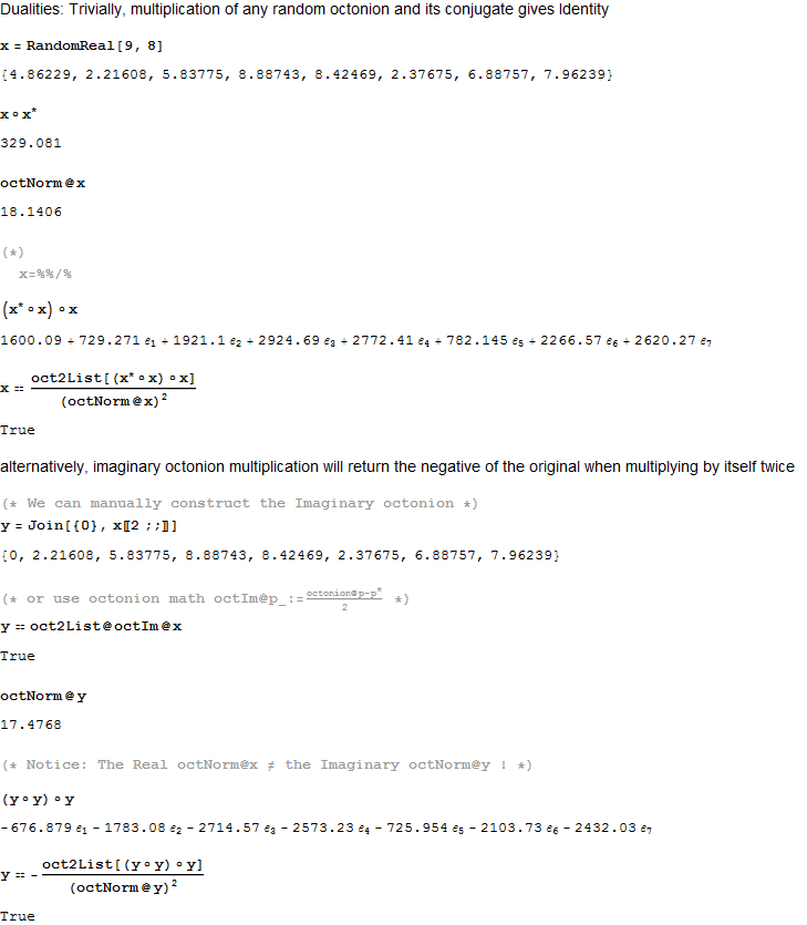
Octonion triality testing
I am working on validating some theoretical work on the triality automorphisms of the split octonions. This is a post with preliminary work on that… for those who are interested 🙂
BTW – It requires the here.
An addendum to the original post (below):
[WolframCDF source=”http://theoryofeverything.org/TOE/JGM/octonion triality checks.cdf” width=”900″ height=”8000″ altimage=”http://theoryofeverything.org/TOE/JGM/octonion triality checks.png” altimagewidth=”900″ altimageheight=”8000″]