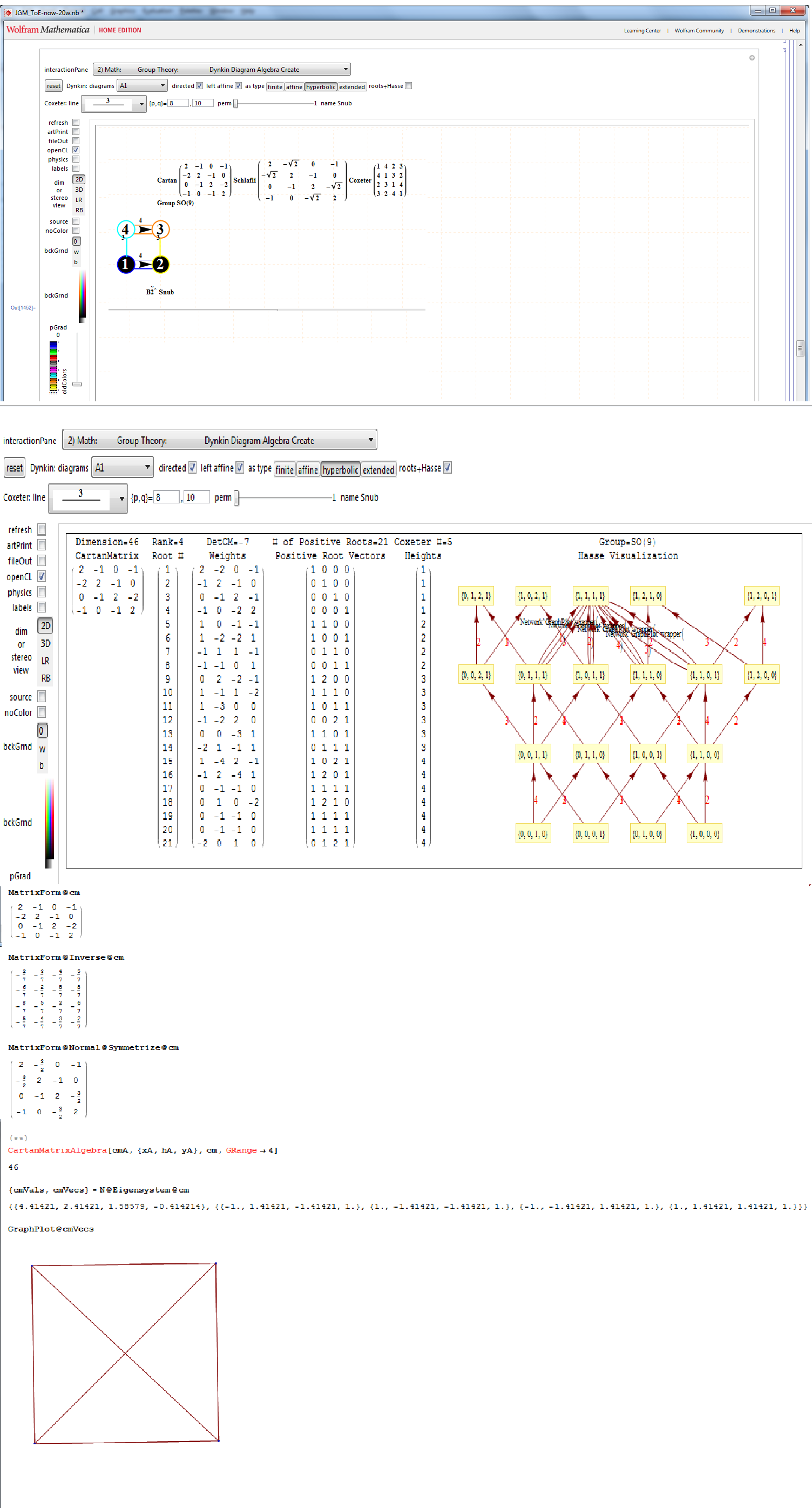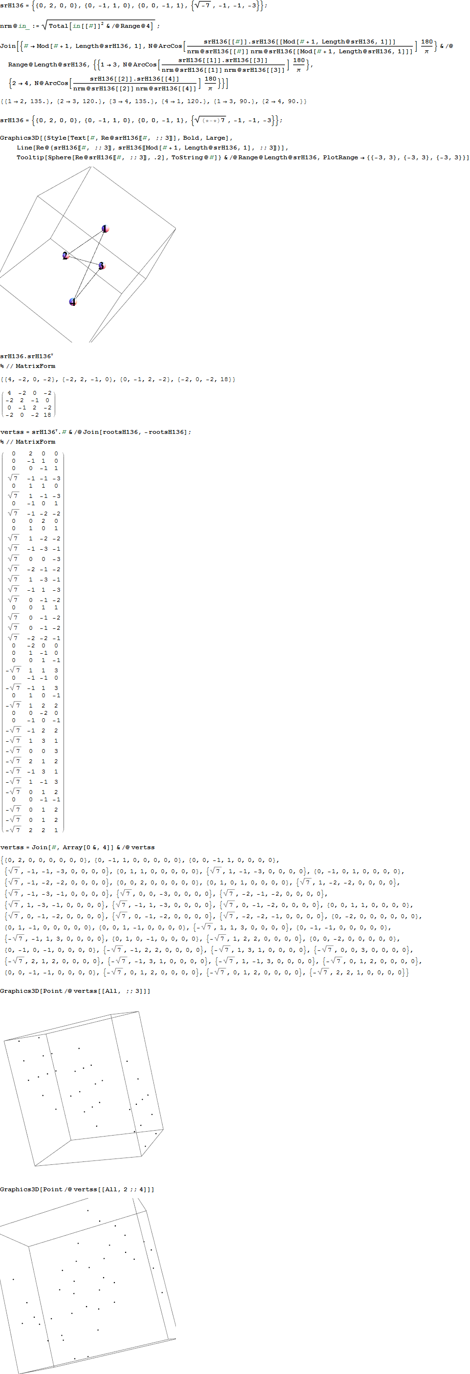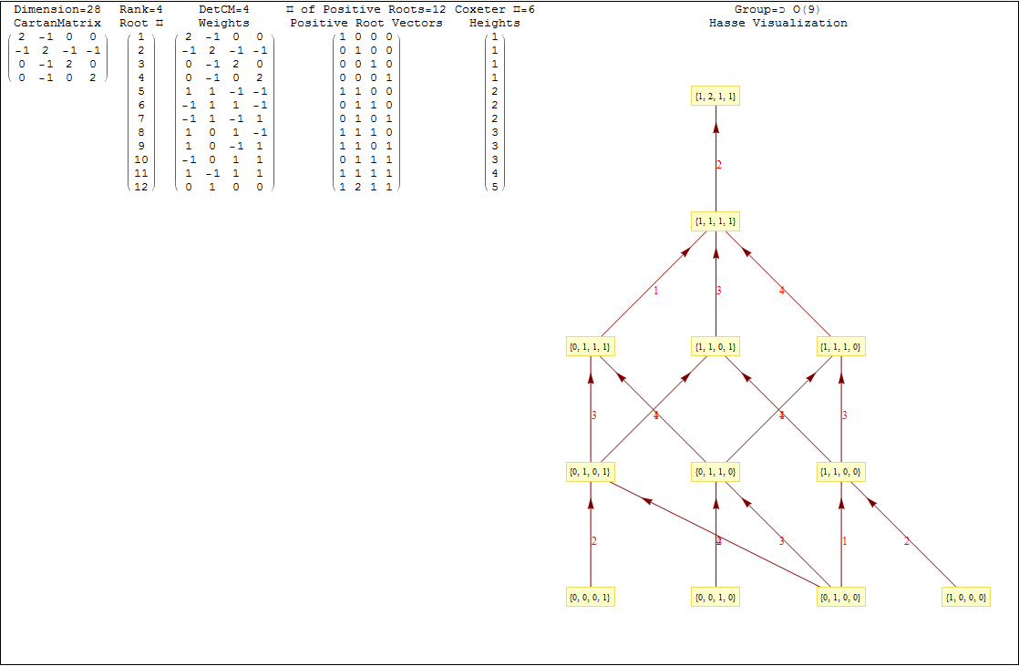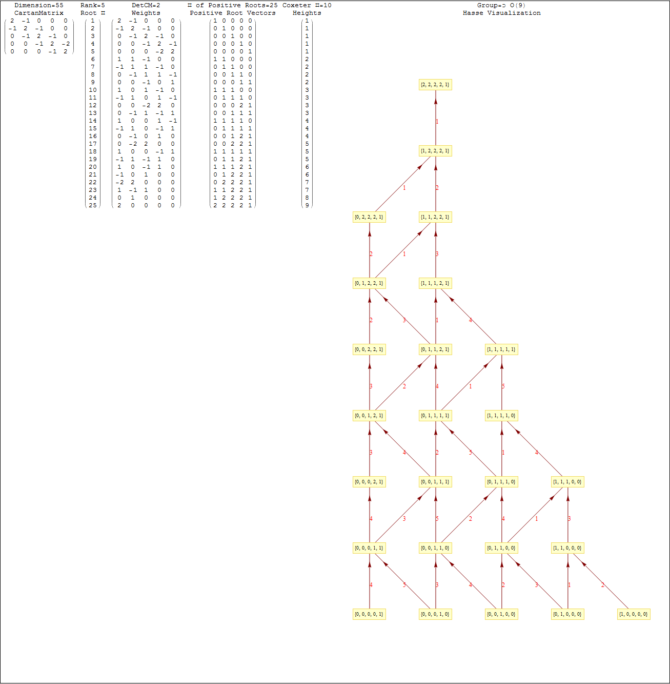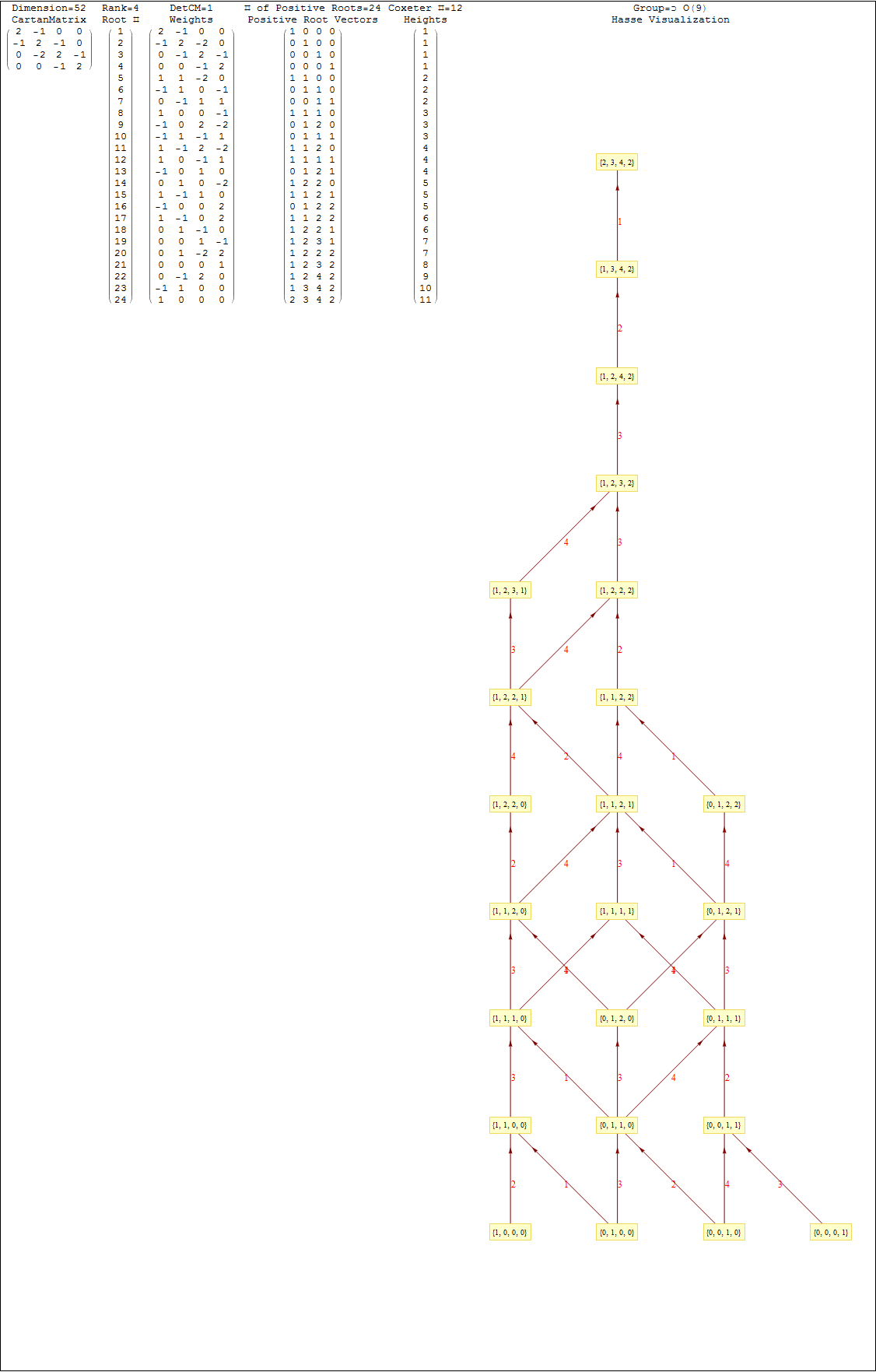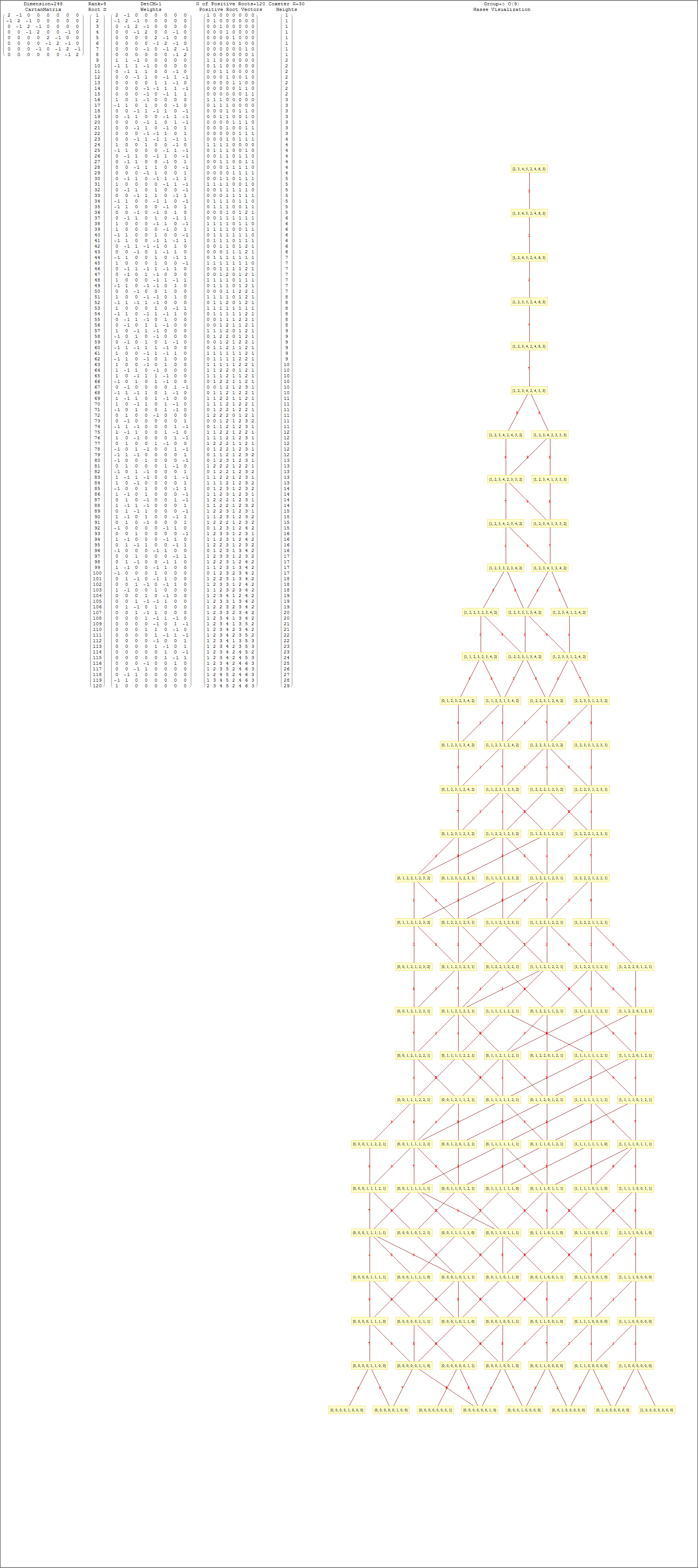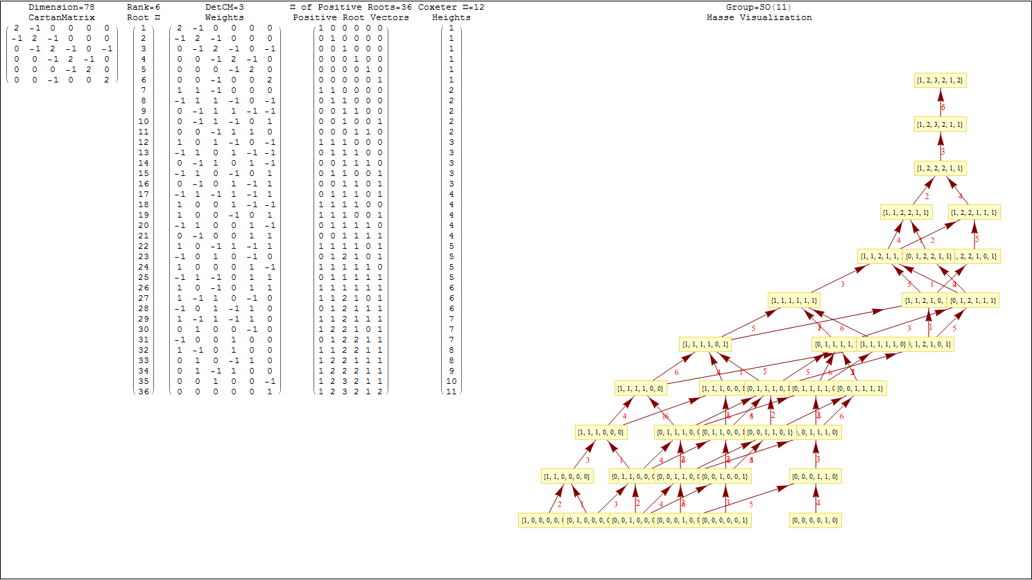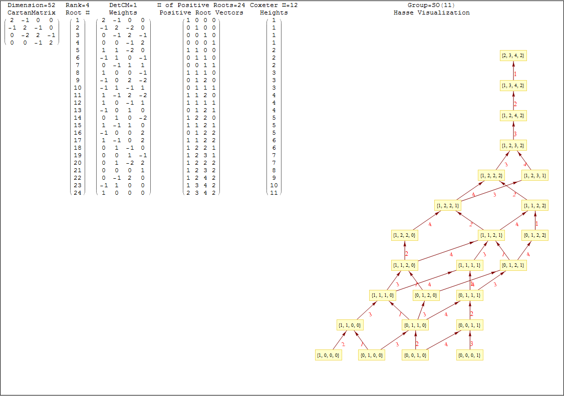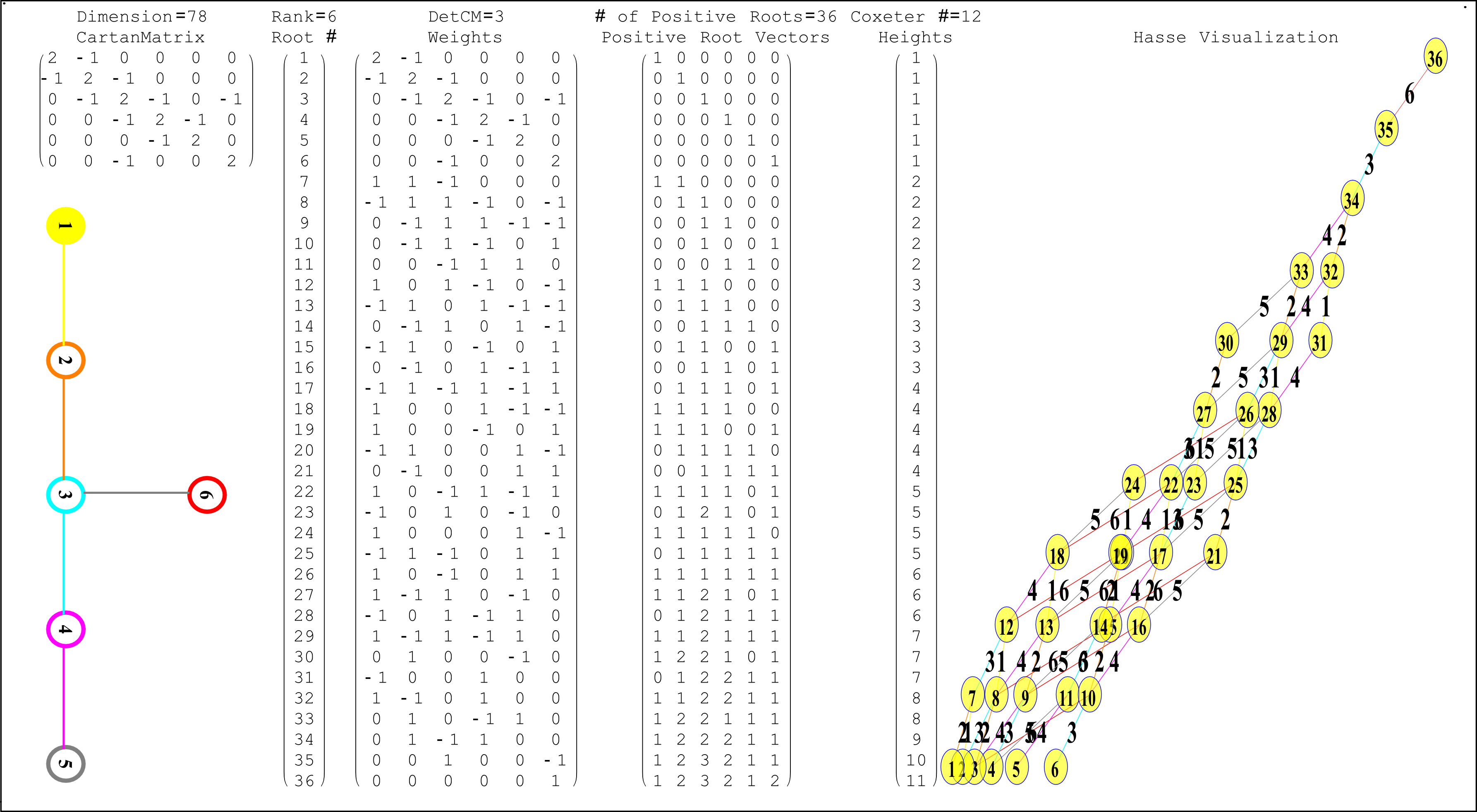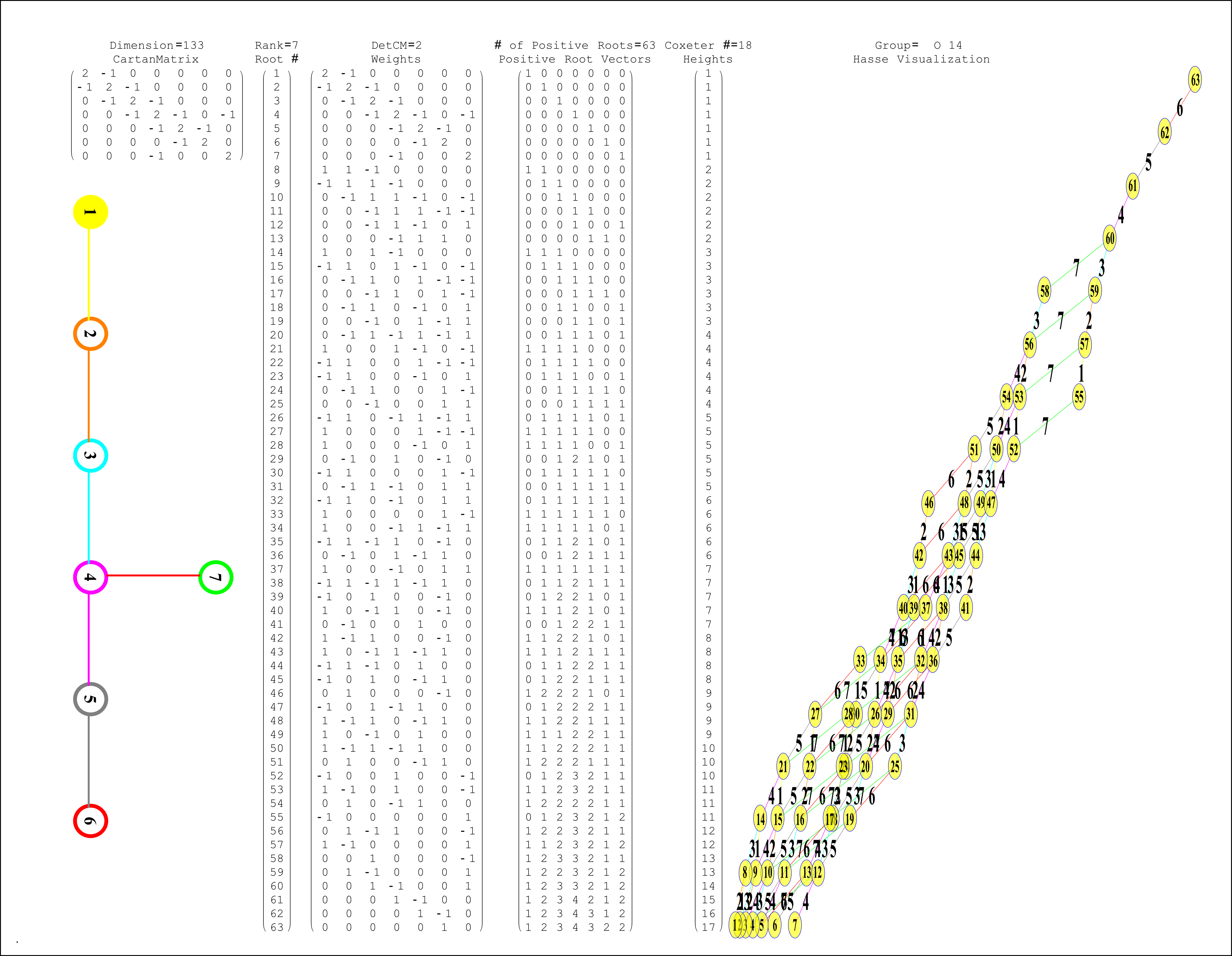
This uses the latest Mathematica version 13.2 with code tweaks to better understand what is being presented, including the E8 Algebra roots, weights, and heights. This is used on the E8 group theory page of WikiPedia.

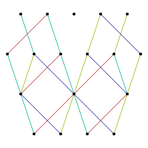
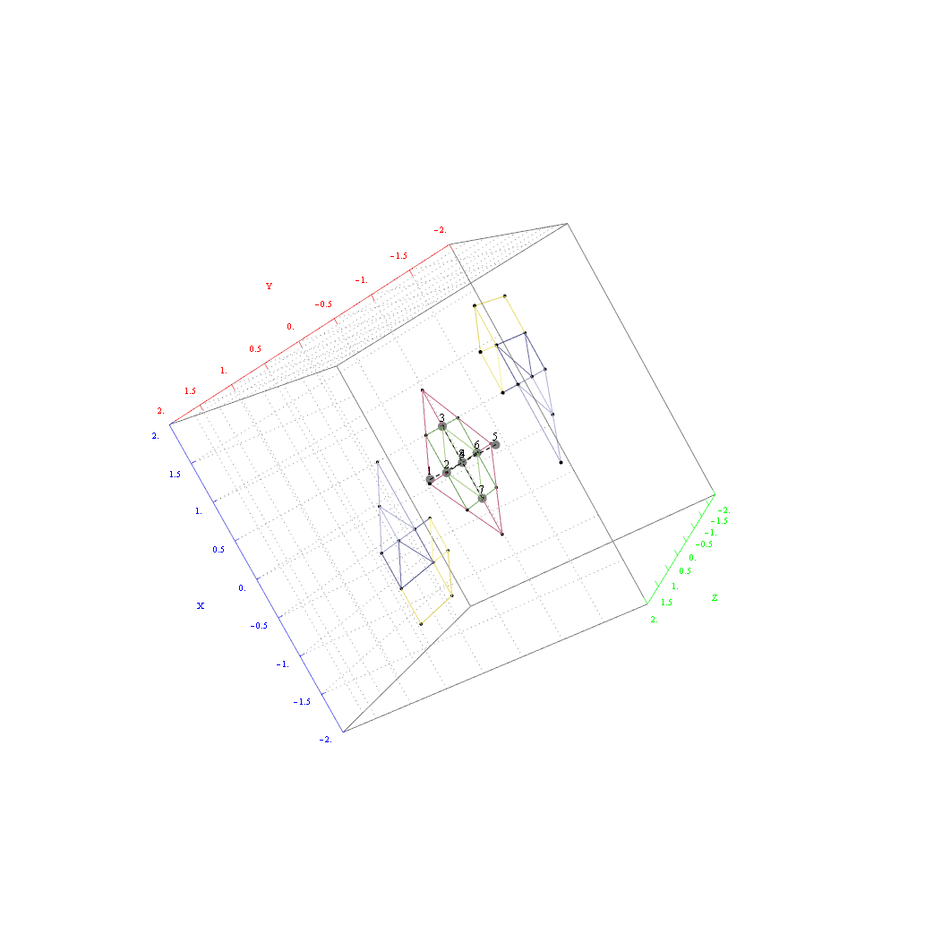
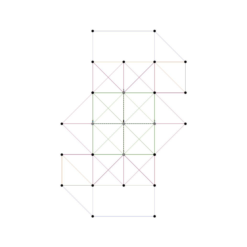
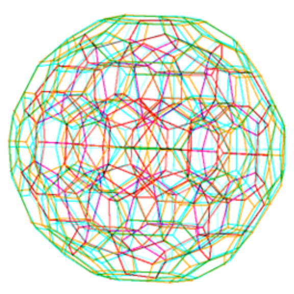
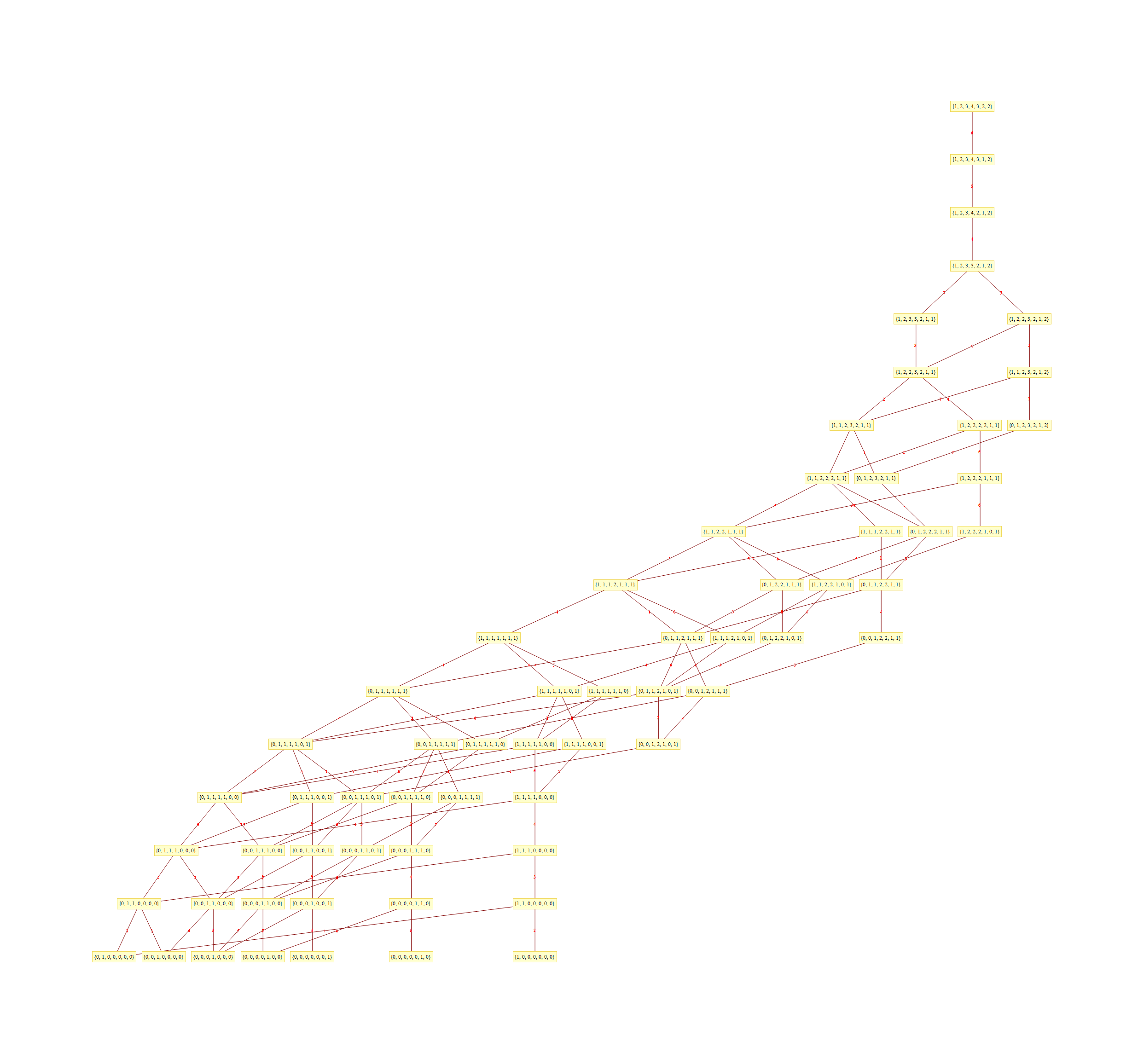
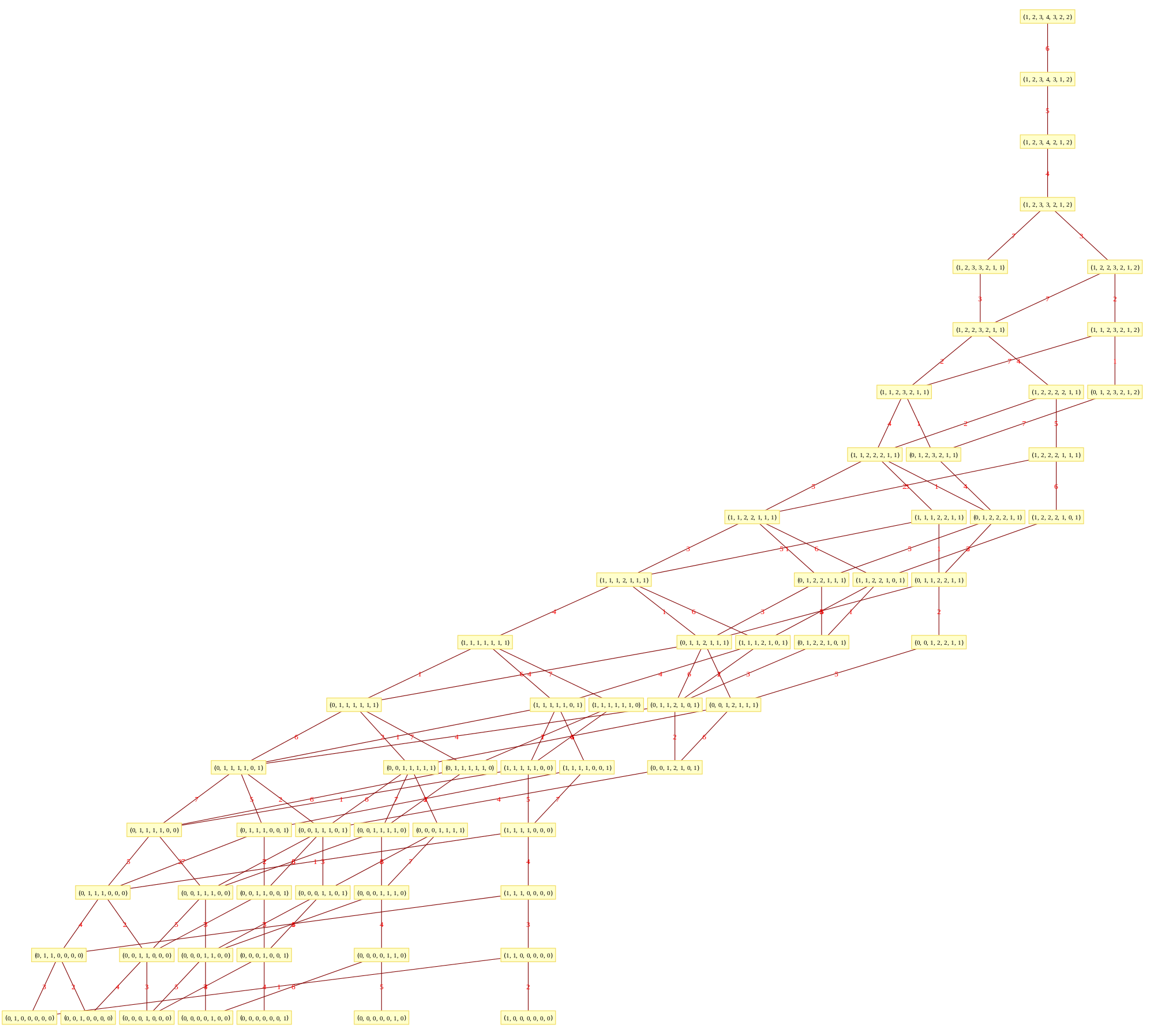
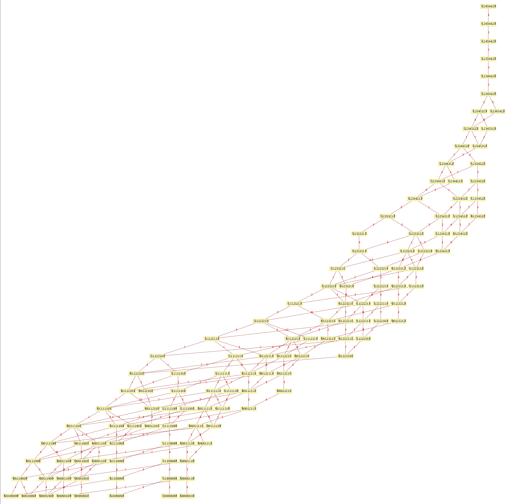
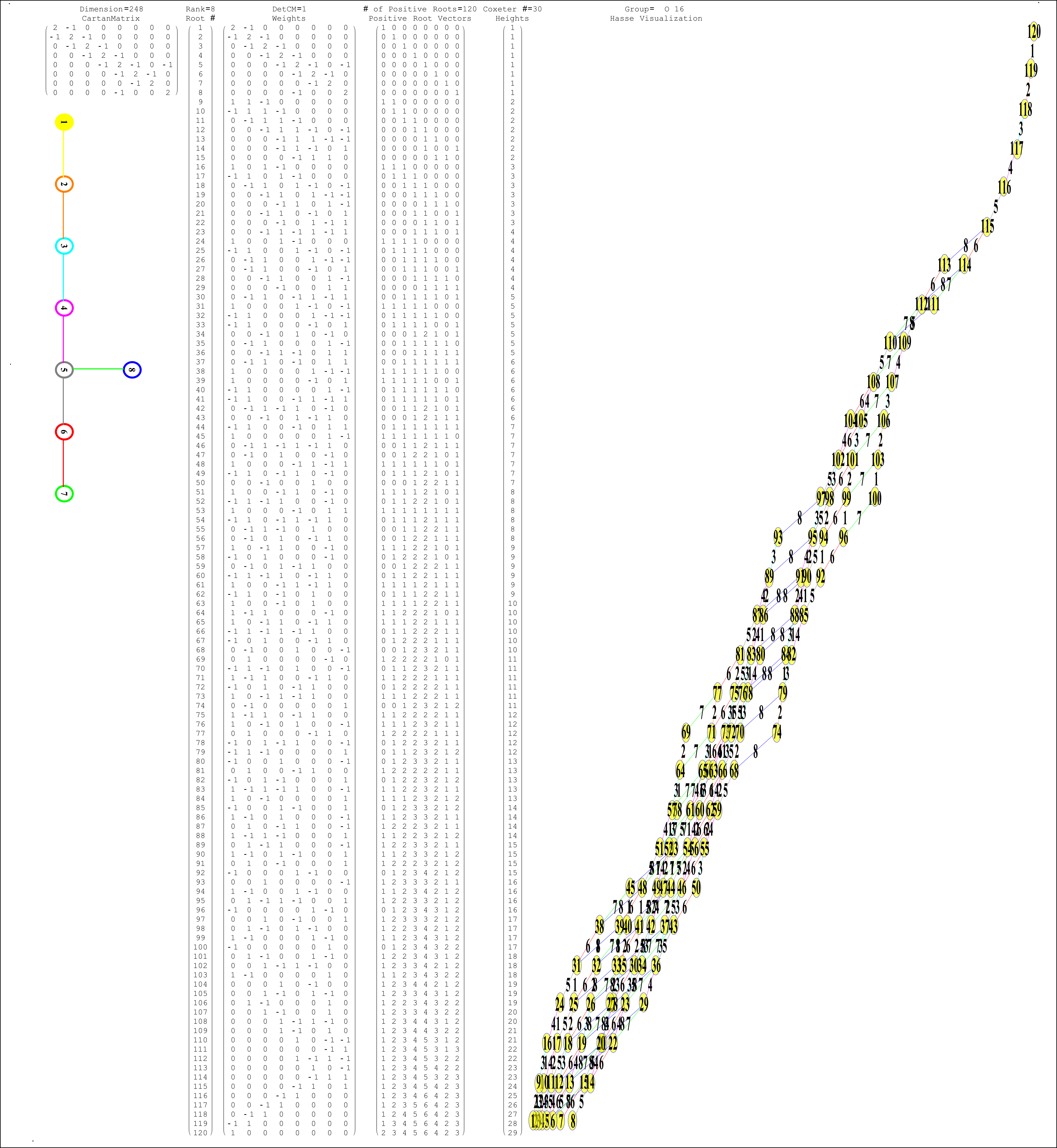
For a more graphic intensive E8 Hasse visualization, see below with both positive and negative roots and more node information and graphics. See here and here for the Mathematica notebook and PDF respectively.