Category Archives: Physics

The Beauty of Roots

For a nice introduction to roots and their fractal nature, see this post from 2011 on John Baez’s Azimuth blog or his 2023 UCR page here. Some of my code here is sourced from a great repository of interesting math visualizations from many others including the author of the pywonderland GitHub of Zhao Liang.

The SVG images below can be clicked to zoom in on another tab, but here is a Mathematica Notebook with Tooltip info on the selected roots. That SVG is 8000×8000, so you may have to <cntrl>- to zoom out to see any of the interesting parts (depending on your screen resolution and browser setup).
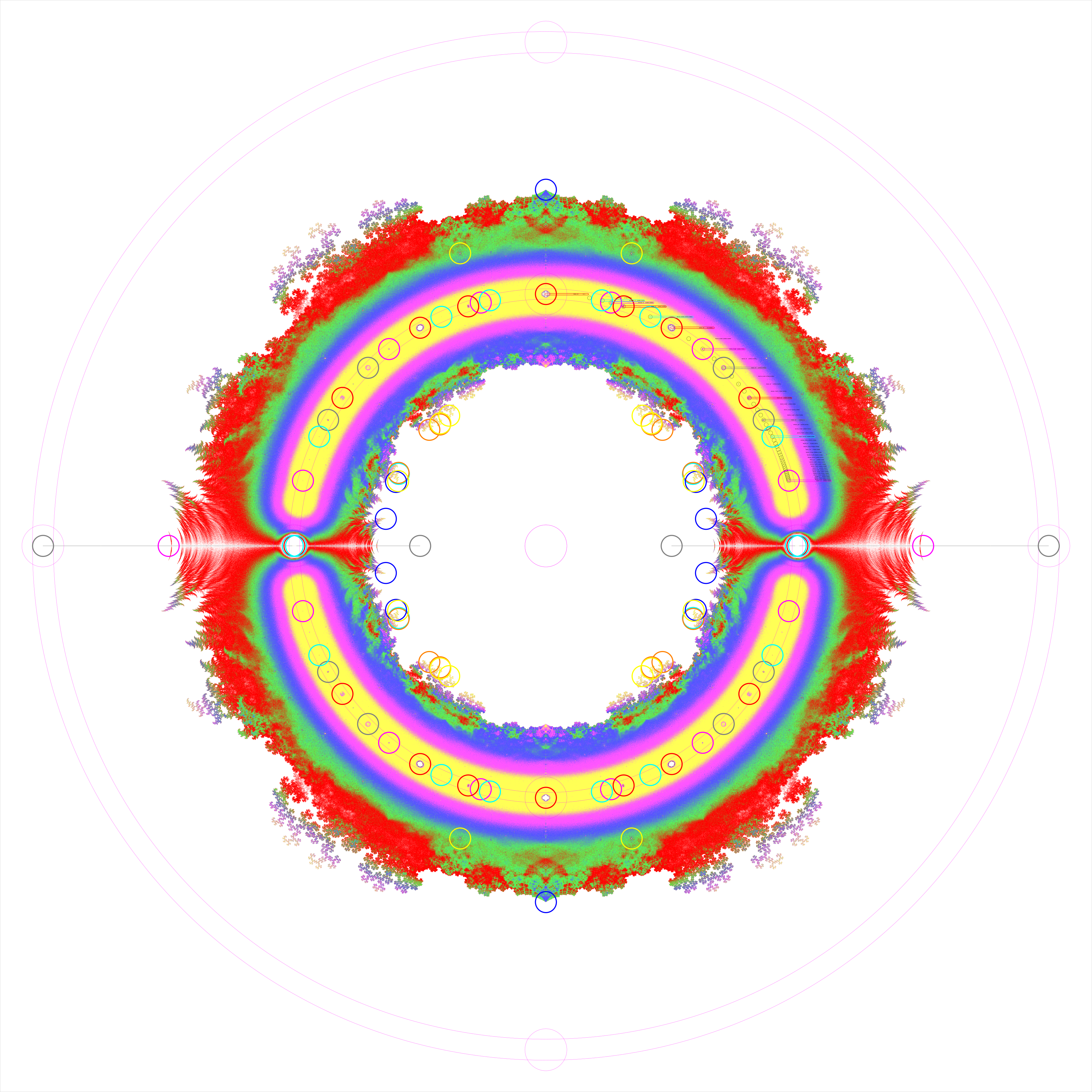
All roots of polynomials up to 224 (~16.7 million) with +/-1 coefficients.

The roots are complex valued (Real x-axis and Imaginary y-axis) with normalized binVal(ue) defining the color from 0 to 1. The ColorRules are as follows:
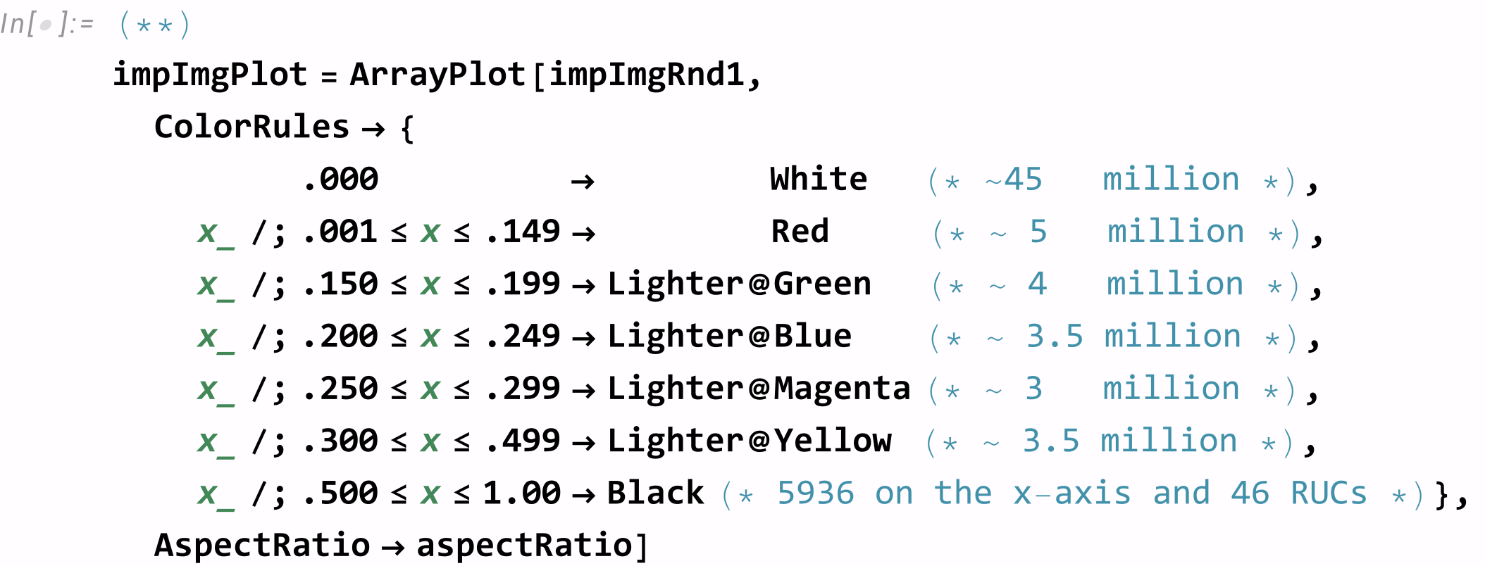
A binVal{x,y} is incremented when the {x,y}={Real,Imaginary} root elements fall in that particular bin. The results are normalized by dividing each bin by the Log2@binVal{x,y} / Max@Log2@binVal. So the two x-axis binVal={+/-1,0}width/2 have a binVal=1 means the cumulative roots in every degree have the most roots at that 0/π location. The two y-axis binVal={0,+/-1}height/2 have a binVal of ~.903 that land in those  +/-i π/2 bins.

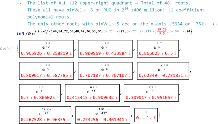
The analysis below provides more detail on the Roots-of-Unity Circle (RUC) at the center of the light yellow area. These are interesting in that there are 4 quadrants each with 12 roots that all have 1/2< binVal <1 at the center of holes.

There are 6 roots that sit in holes surrounded by zeros (i.e. 2π/{12,10,8,6,5,4}) and 6 roots in holes with surround values <1/2 (i.e. 2π/{24, 14, 7, 11/2, 29/6 (75°), ~437/90 (77°)}). The only other binVal roots >1/2 are on the 1 pixel wide x-axis with 5936 of 8000 (~75%) from the x-y grid of 8000×8000 (64 million) bins which sum over each of the 224 (~16 million) roots-of-polynomials with -/+1 coefficients. The rest of the x-axis roots are 2020 bins equal to 0 and only 44 bins between 0 and 1/2).
The large table below shows 100 detail areas of “special” algorithmically selected locations from bin location Tally counts of 7732 unique binVals. About 50% of these occur in 2 to 4 (symmetric) locations with a binVal>1/2. The other 50% of the Tally counts have binVal<1/2 and tend to have 103 to 106 locations with all but 5980 (of 64 million) bins. This is made clear from the above MatrixPlots.

Each detail area shows a 400×400 ArrayPlot around the selected location and an 11×11 zoom-in of that binVal matrix with its ArrayPlot. They include the 48 RUC roots and 12 x-axis roots with binVal>1/2, and 40 off-axis roots with ~2/3 bins of zero and 1/3 with binVal<1/2. This off-axis list includes one set of 4 quadrant roots that is a proper hole (in the 4 yellow rings located just above/below the bottom/top apex in the full image or 10-14th from the bottom in the detail list below). The other 9×4 roots are what I call “pseudo-holes” that have no enclosed high central binVal.
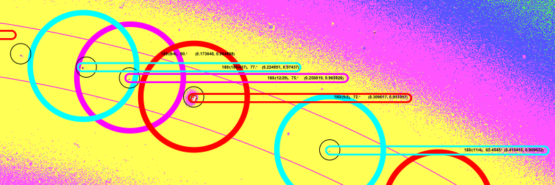
Zoom-in of detail in the upper-right quadrant RUC root values – click SVG to create another tab and zoom in your browser.

The annotated upper-right quadrant of the SVG image has the RUC roots ringed in colors (shown in the zoom-in graphic above) with large colored rings assigned by their binVal. Annotated rings with binVal>1/2 are cyan, magenta, and red. The binVal<1/2 are yellow, orange, or blue rings. The smaller black ring is what is visible in the 11×11 MatrixPlots below. To the right is the text with the angle at which the root is located.

FYI – The color scheme on these detail zoom MatrixPlots are set to the default in order to maximize and highlight the numeric differences, so they don’t match the ColorRules in the large 8000×8000 MatrixPlot at the top of the page.

Click the image below to see this SVG and zoom further.

Detail areas of special roots with a 1000×1000 ArrayPlot and an 11×11 zoom of the Abs root values and its ArrayPlot

Improved SVG E8 Petrie and Hexagonal Triality Representations

Stay tuned for more images. I think I will use this post to place my more beautiful works!
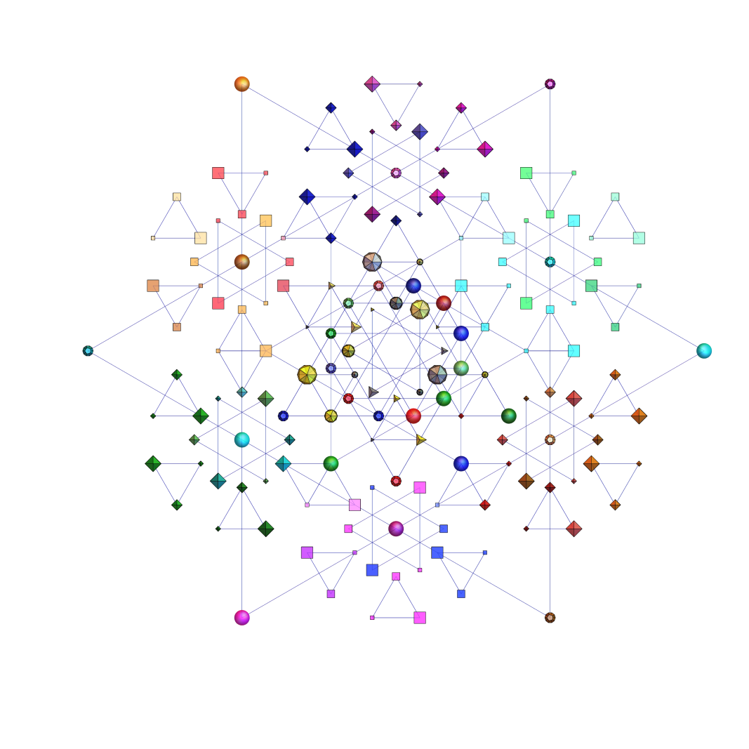
E8 in Petrie projection with 3D theoretically assigned physics particles

These use a better combination of specularity and opacity with both math and physics (theoretical assigned) 3D vertices. This is accomplished by actually projecting into 3D but using only X-Y basis vectors with Z={0,0,0,0,0,0,0,0} and the (virtual) camera at XYZ={0,0,}.

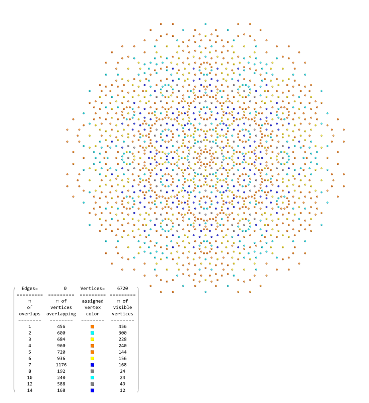
Some images use color coding for vertices that indicate overlaps (e.g. when in the spherical (math) vertices E8 hexagonal basis). The overlap number data may then be presented in the lower left. This data can be removed using SVG editors such as Inkscape.

Some images also show the 3D technical axes (basis) projection vectors as well as the vertex, edge, and other data. Also, bear in mind that the PNG images shown below (so they are visible in Google Images after being crawled) tend to show pixelation artifacts and can present with black background vs. white. The SVG presentation (obtained by clicking the embedded image link) will be correct and the transparent background can be modified easily (e.g. with Inkscape).

Please note, these are provided under Creative Commons CC BY-SA 4.0 Attribution-ShareAlike 4.0 International license, so if you use them please cite me at this site (or me on the Wikipedia (WP) article or WP commons source):

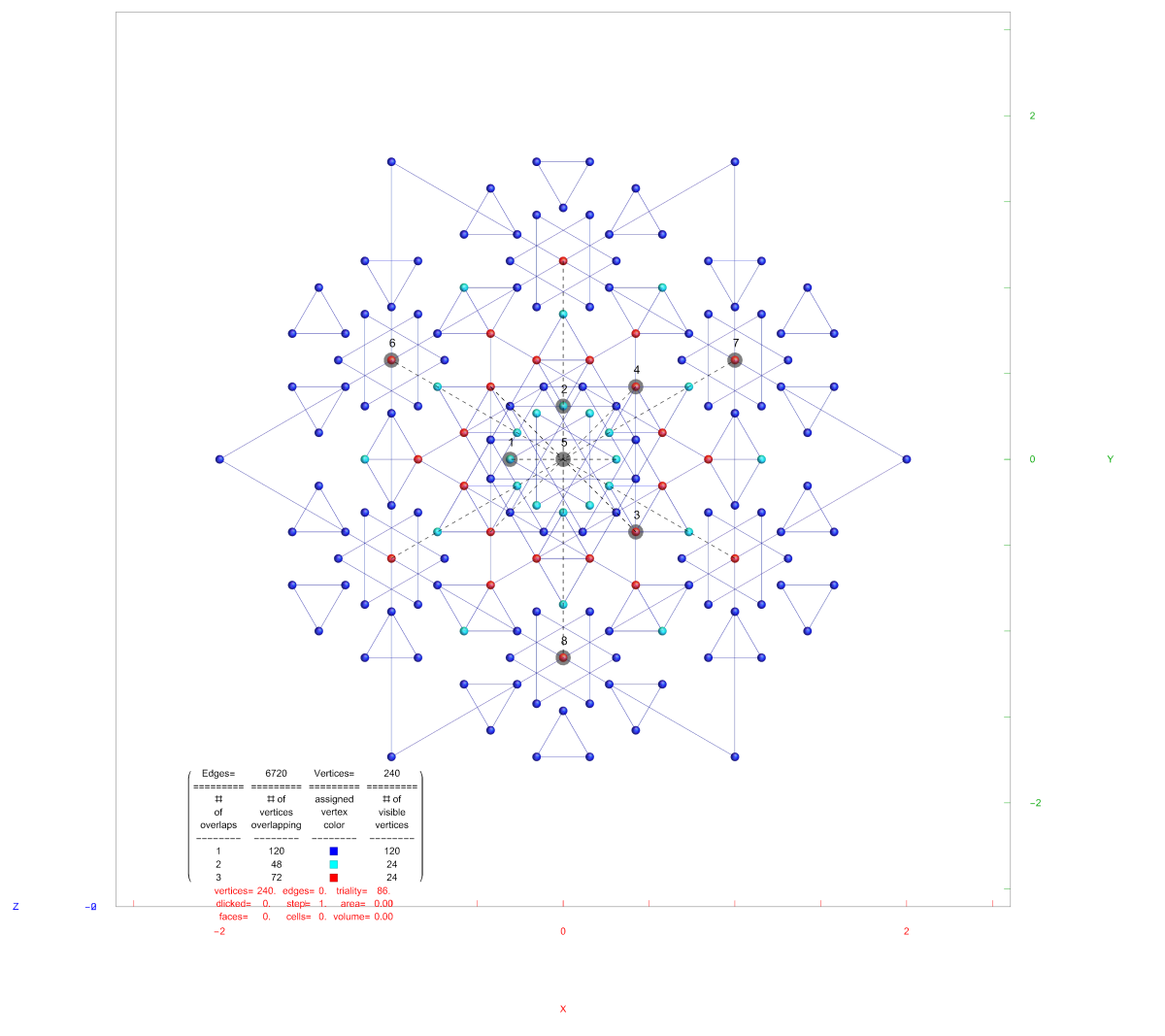
Below is the well known PR photo for E8 in Petrie projection with basis vector axes and data presented (click the image for the downloadable SVG):

E8 in Petrie projection with axes and other data

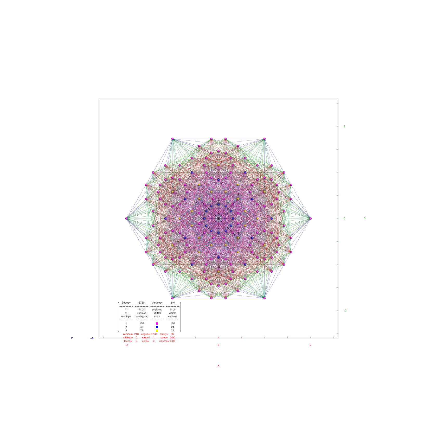
Below is the E8 hexagonal (aka. as the “E6/D4 Mox [6]” in Wikipedia) projection:

E8 hexagonal (aka. as the “E6/D4 Mox [6]” basis in Wikipedia) projection

The E8 hexagonal with the 3D assigned theoretical physics vertices:

E8 with the 3D assigned theoretical physics vertices in hexagonal projection

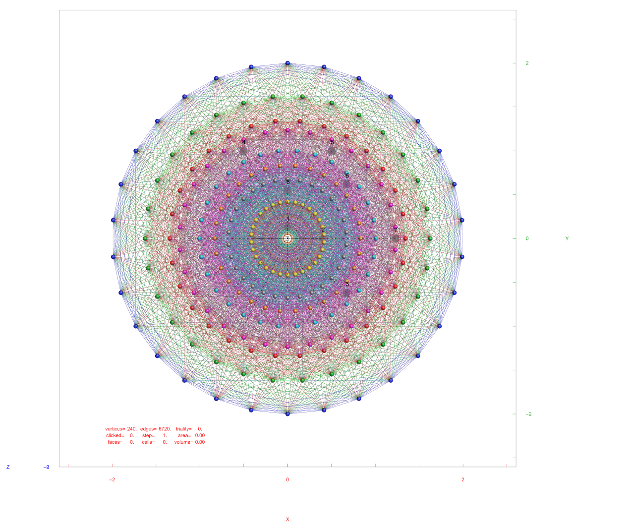
The E8 hexagonal projection with 6720 edges:

E8 with edges in hexagonal projection

The Rectified E8 in hexagonal projection with 6720 vertices:

Rectified E8 with edges in hexagonal projection

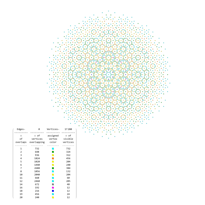
E8142 in hexagonal projection with 17280 vertices:

E8142 in hexagonal projection

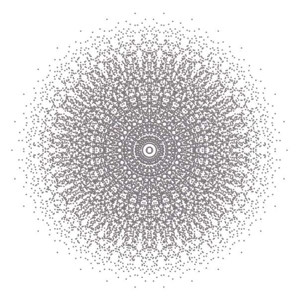
E8142 in Petrie projection with 17280 vertices:

E8142 in Petrie projection

The periodic table with orbitals in 2D:

The periodic table with orbitals in 2D

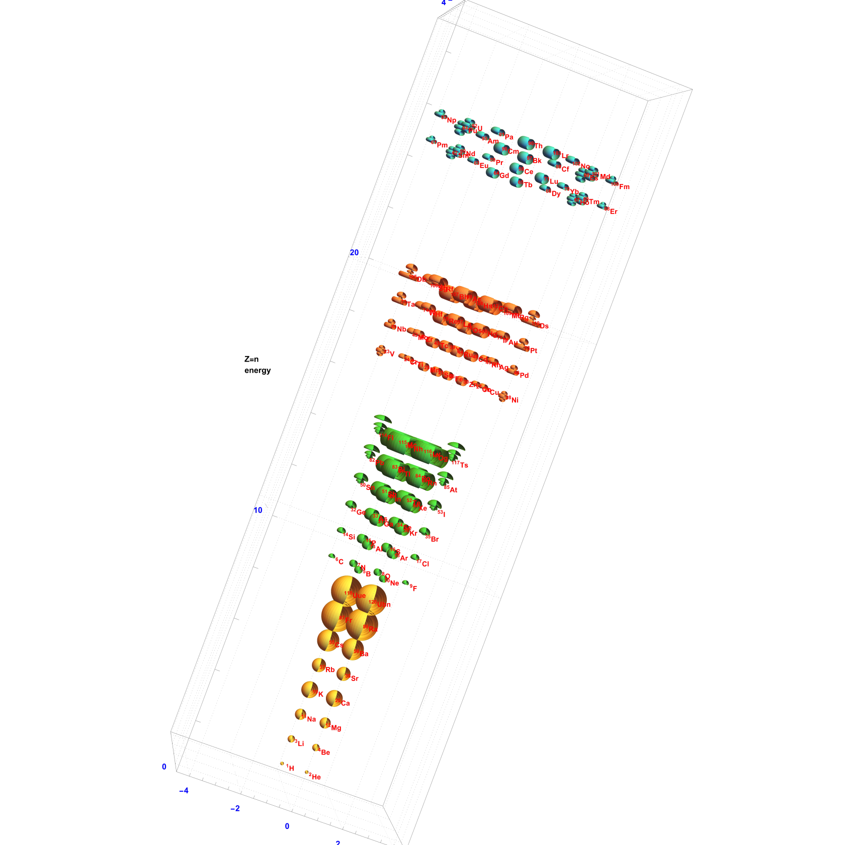
The periodic table with orbitals in 3D:

The periodic table with orbitals in 3D

Kneser neighborhood graph of Niemeier lattices with associated Mathematica Notebook here:

Kneser neighborhood graph of Niemeier lattices with associated Mathematica Notebook here.

The E8 subgroup tree:

E8 Subgroup Tree with associated Mathematica Notebook here.

Riemann Zeta function zeros:

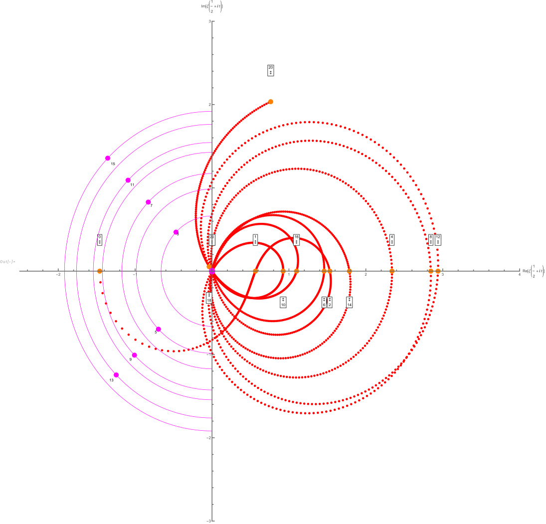
This is a polar plot of the first 20 non-trivial Riemann zeta function zeros (including Gram points along the critical line ζ(1/2+it) for real values of running from 0 to 50. The consecutive zeros have 50 red plot points between each with zeros identified by magenta concentric rings (scaled to show the relative distance between their values of t).
All roots of polynomials up to 224 (~16.7 million) with +/-1 coefficients.
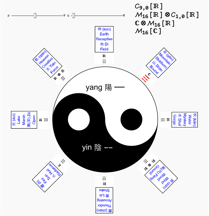
Bott Periodicity Clock of Cl(9,0) as it relates to the Hopf Fibration of CP4

E8 and H4 Gram Matrix Visualizations

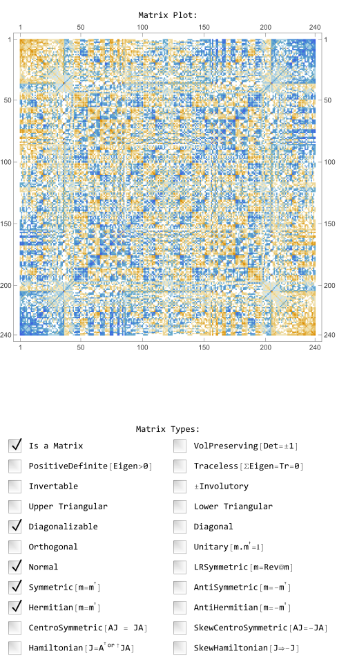
Beautiful MatrixPlot’s of E8 and H4.

This is not the typical E8 Gram matrix representation as the Cartan matrix using only the simple roots (shown at the end of this post).

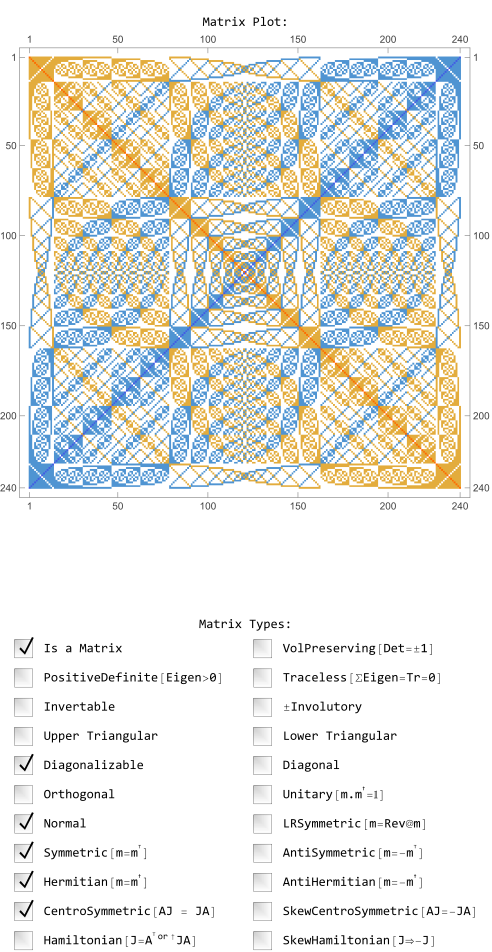
It uses all 240 E8 vertices (+120/-120 roots) of the E8 Split Real Even (SRE) vertices to produce the Gram matrix (with vertices sorted in simple numeric order):

Full E8 Split Real Even (SRE) vertex Gram matrix in vertex numeric sort order

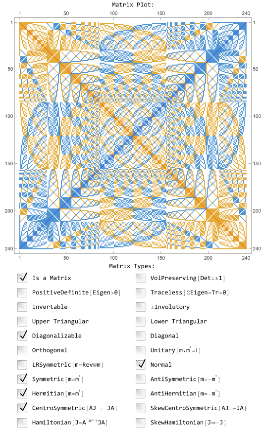
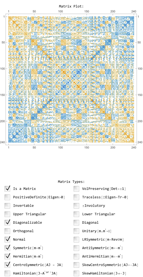
The same 240 E8 vertices (+120/-120 roots) below are sorted by the 9th row of the binary structure Pascal Triangle, excluding the 2nd & 2nd to last entries of -/+ 8 (i.e. {-1,-8,-28,-56,70=(-35/35),56,28,8,1}, where the 112 integer D8 are -56/56 and the 128 half-integer BC8 are {-1,-28,-35,35,28,1}).

Full E8 Split Real Even (SRE) vertex E8 Gram matrix in Pascal Triangle order

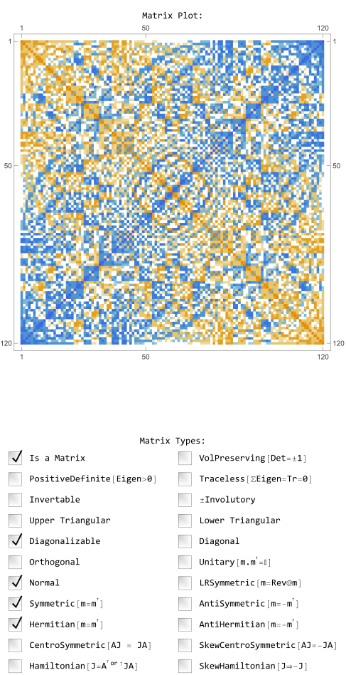
As above, but with H4+H4φ 8D Gram matrix created using the dot product of E8 against the 8×8 E8 to H4 folding matrix U:

H4+H4φ 8D Gram matrix

Now with only the H4φ 4D Gram matrix created as 120 H4 4D vertices:

H4φ 4D Gram matrix

Compare this to the Gram matrix using the root weights of E8 (in Pascal triangle order vs. sorted into root and/or weight order):

E8 Gram Weights (in Pascal Triangle order)

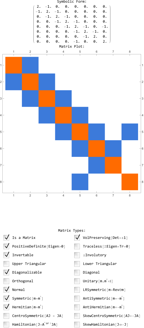
Then compare to the Cartan matrix produced as the Gram matrix of only the 8 E8 simple roots:

E8 Cartan matrix from 8 simple roots

Mathematica Analysis of JLN’s TUFT

This post presents my independent analysis of Jenny Lorraine Nielsen’s (JLN’s) Topological Unified Field Theory (TUFT). It symbolically implements her equations related to the fundamental constants, General Relativity (GR) cosmological parameters, and Standard Model (SM) particle masses and magnetic gyrometric ratios and anomalous moments. It then calculates the values and compares them against the PDG CODATA from Wolfram’s curated data sets.

The structure of this analysis is shown (below) in PNG (click for SVG version) or see here for the full PDF of the analysis or here for the Mathematica Notebook (NB) version:

Outline of my Mathematica analysis of JLN’s TUFT predictive theoretical parameters
E8 Hopf Fibration
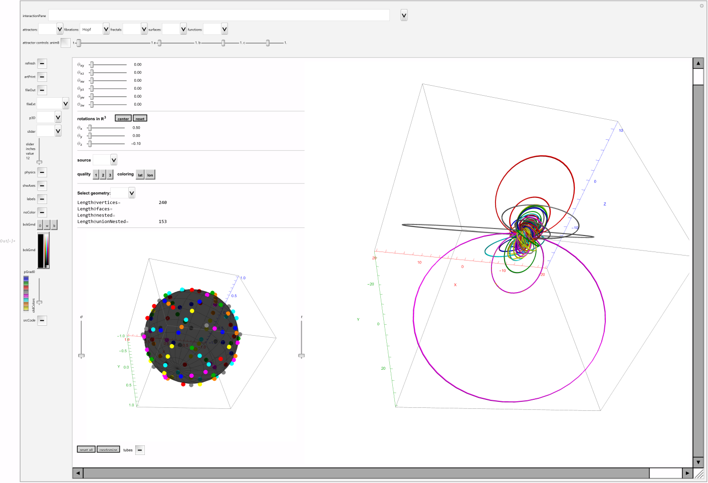
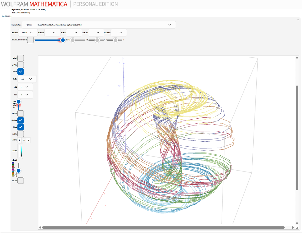
The Aizawa Chaotic Attractor

This is all also related to the Clifford algebra of Cl(9,0) with the Bott Periodicity clock showing the related algebras (click for SVG):

Bott Periodicity Clock of Cl(9,0) as it relates to the Hopf Fibration of CP4

The Bott periodicity clock uses a Mod 8 clock face with second hand mnemonics taken from the I-Ching with the real Clifford algebra of signature (p,q) denoted as Clp,q(R)=Cl(p,q). An animated (GIF) example is on the Bott Periodicity Wikipedia page.

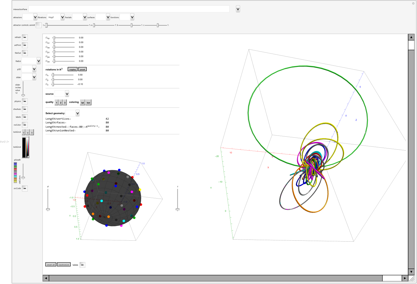
E8 and H4 Hopf Fibrations with the Aizawa Chaotic Attractor

If you are working with topological field theoretic Hopf fibrations, chaotic attractors, and/or E8 and any of its extensive set of maximal subgroups, polytopes, lattices and codes or its folded (rotated) H4 family of polytopes (e.g. 600 and 120 cells in their vertex, cell, face, and edge orientations), VisibLie_E8 can group theoretically integrate all of these concepts visually!

Click on the PNG image to get the SVG version.

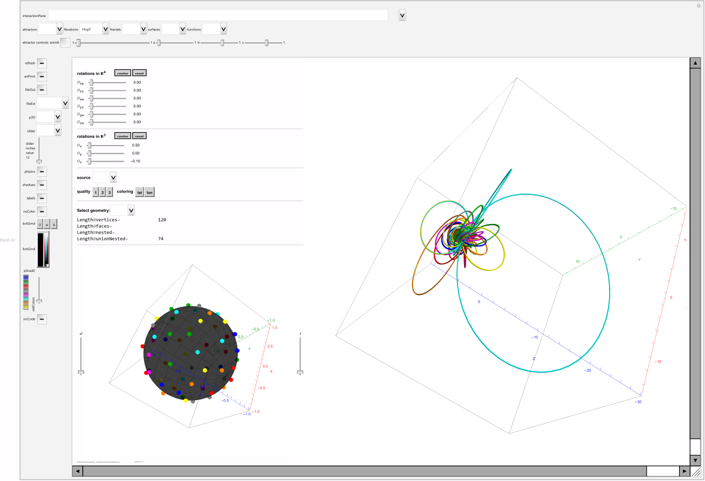
E8 Hopf Fibration
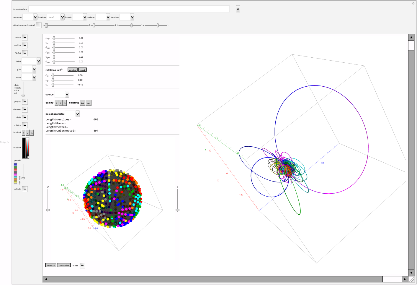
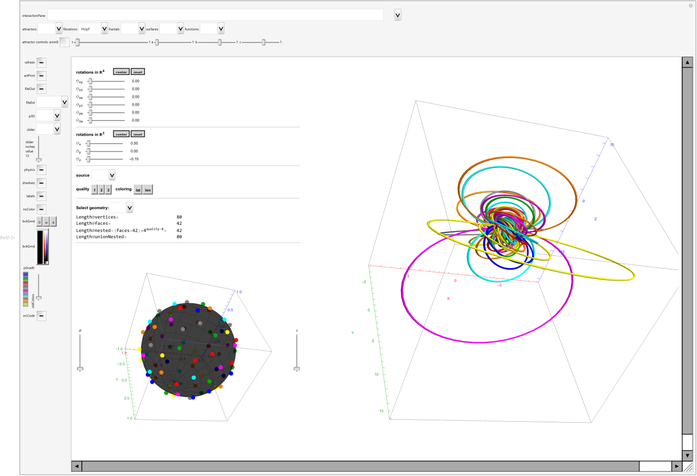
H4 600-cell Hopf Fibration
The H4 cell-first {5,3,3} 120-cell Hopf Fibration (with envelope of a Chamfered Dodecahedron)
The Aizawa Chaotic Attractor

This is all also related to the Clifford algebra of Cl(9,0) with the Bott Periodicity clock showing the related algebras (click for SVG):

Bott Periodicity Clock of Cl(9,0) as it relates to the Hopf Fibration of CP4

The Bott periodicity clock uses a Mod 8 clock face with second hand mnemonics taken from the I-Ching with the real Clifford algebra of signature (p,q) denoted as Clp,q(R)=Cl(p,q). An animated (GIF) example is on the Bott Periodicity Wikipedia page.

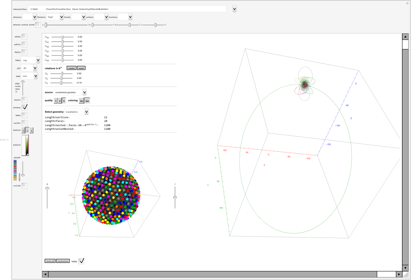
A few more Hopf geometries:

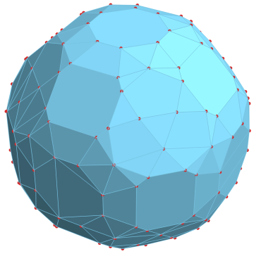
The envelope of the vertex first 600-cell aka. PentakisIcosidodecahedron
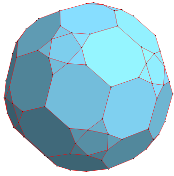
The envelope of the cell first 120-cell aka. Chamfered Dodecahedron
The Icosahedron @ quality 3

Comparing the new and older forms of my E8 to H4 folding matrices

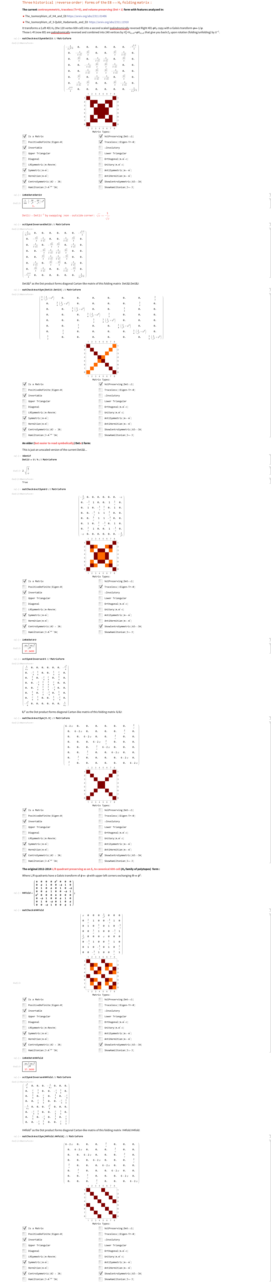
If anyone is using my E8 to H4 folding matrix in their research, this post provides a bit of context from the original form (2012-2014) as it was improved to the current form. Drop me an email if you are using my work or have questions, or find errors, etc.

See here (Baez), here (Castro-Perelman), here (Schmidt), here (Ruen on WP E8 Polytope D4-E6 “Mox” projections) for properly cited examples.

I am working with a few who are using my work on cryptography, quantum computing, and computation optimization, but they have yet to post or publish results.

Of course, many authors may or may not be aware of their use of my prior art (so it goes without citation) e.g. here (Nielsen) using the fine structure constant α-n as a hyper-dimensional geometric nD scaling factor for the fundamental constants, such as my definition of a new Unit of Measure (UoM) distinct from Natural Units from 1998-2001).

The image below is also available as a Mathematica notebook (NB) or PDF. Click the PNG image for the SVG version.

The first part reviews the current Hermitian, centrosymmetric, traceless (Tr=0), and volume preserving (Det = 1) form of the folding matrix (U).

The last part reviews the traceless Hermitian unitary matrix (uU) of determinant 1 (i.e. A7=SU(8)) with characteristic polynomial |coefficients| of the 5th row of the Pascal triangle (1,4,6,4,1}. This matrix has the same characteristic polynomial as that of the 3-Qubit Hadamard matrix. Both are related to QM Hadamard, CNOT and SWAP gates and Pauli matrices from which it, cmU, and U are constructed.

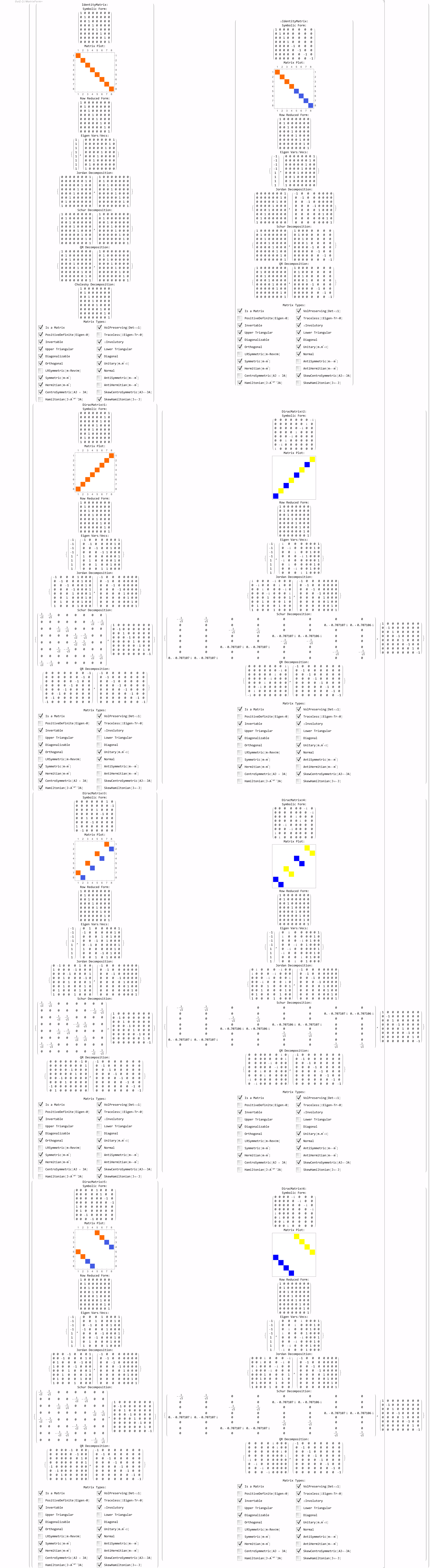
Below that is another matrix analysis of the 6 8×8 Dirac matrices (i.e. DiracMatrix[#, Dimension -> 6]&/@Range@6) with the Identity and +/- Traceless Identity matrices prepended. These have similar properties to uU with the addition of being (skew)Hamiltonian matrices.

Comparing E8 to H4 folding matrix versions
Matrix Analysis of Identity and Dirac Matrices

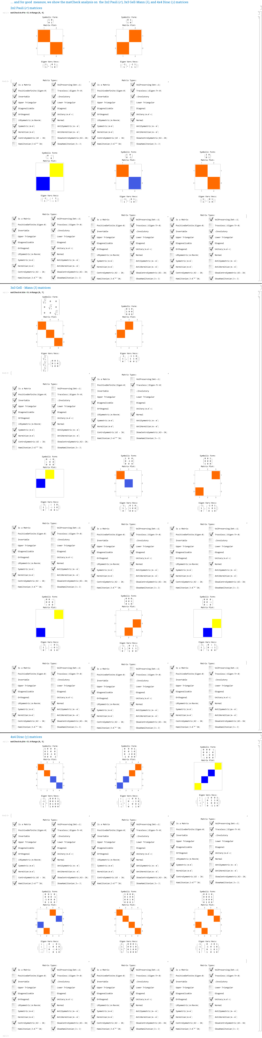
Now for good measure, we show the matrix characteristics of the 2×2 Pauli, 3×3 Gell-Mann, and 4×4 Dirac matrices:

Matrix Analysis of 2×2 Pauli, 3×3 Gell-Mann, and 4×4 Dirac Matrices

And finally, we analyze the 8×8 Dimension 6 n=4 Dirac Matrices:

8×8 Dirac Matrices Compare

Mapping Codon:AntiCodon RNA to E8

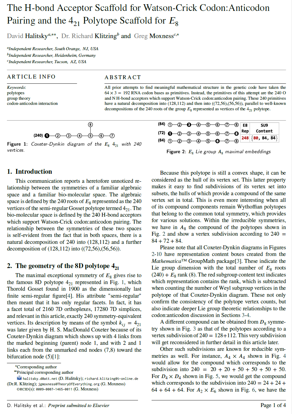
My latest ToE paper here. This paper presents compelling E8 group-theoretic properties that are found in the set of 240 O and N H-bond acceptors which support Watson-Crick codon:anticodon pairing. Empirically correct consequences are deduced from the group-theoretic model.

This paper is related to another recent post here.

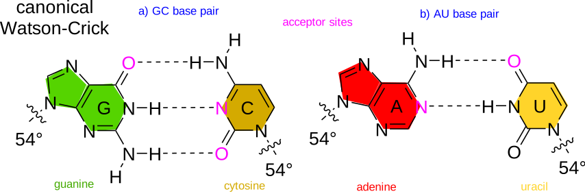
Canonical Watson-Crick RNA Codon Acceptor Sites

Here is the WikiMedia version of the Canonical Watson-Crick Acceptor Sites (Figure 11).

First page – click for the PDF

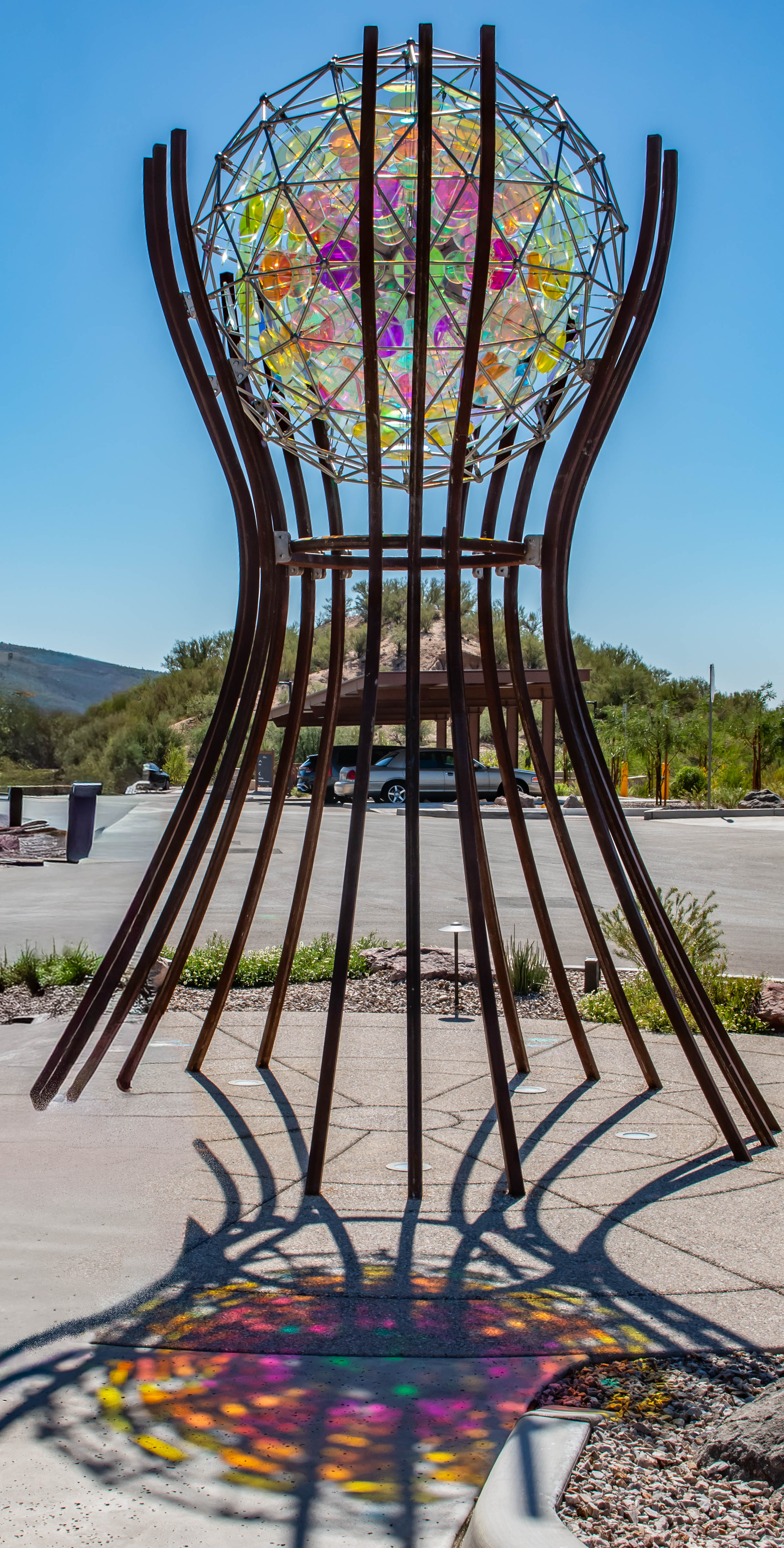
E8 and H4 Stainless Steel and Glass Sculpture in Tucson

Stainless & Glass Public Art Sculpture in Tucson By Ray King.

It’s shape is similar to, but not exactly, a Pentakis Icosidodecahedron, which is 3D the orthographic shadow of the 4D of H4 (and H4φ) 600-cell (s) obtained by folding the 8D object (E8) to 4D. E8 is also known as the 421 polytope.

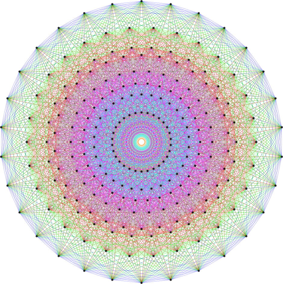
I thought it was interesting that the 2D color shadow on the patio that looks like my E8 diagram called a E8 Petrie Projection:

Jonathan Kirk’s Convex Regular Faced (CRF) Polytope

Links to information on this object are here and here.

Jonathan Kirk’s CRF coordinate permutation

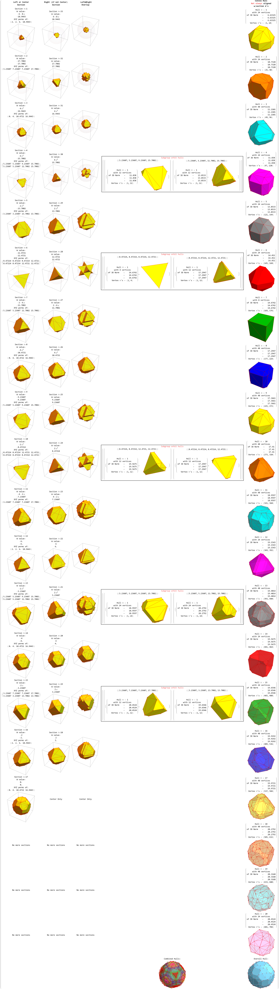
This post used a symbolic permutation list provided in the “rf-poytopes” Polytope Discord discussion thread to produce the Coxeter’s (cell-first, vertex-first, edge-first, and face-first) “simplified” sections shown below.

You can navigate the matrices of links below or simply download the ZIP files for the SVG sectioning for Jonathan Kirk’s Convex Regular Face (CRF) here (40 Mb). The overall convex hull of the cell-first sectioning is similar to, but not the same as, a (496-diminished form of) the H4 BiRectified 600-cell (sectioning of that is shown here).

Overall Convex Hull of the H4 BiRectified 600-cell

For high quality 3D interactive Mathematica Notebook (NB), and SVG or PDF files, you can download them here: NB SVG  PDF

SVG section visualizations:

Orientations for Jonathan Kirk’s  CRF SVG section file links:

              Cell                          Vertex                             Edge                                 Face

MP3 section animations:

Orientations for Jonathan Kirk’s CRF MP3 section animation file links:

              Cell                          Vertex                             Edge                                 Face

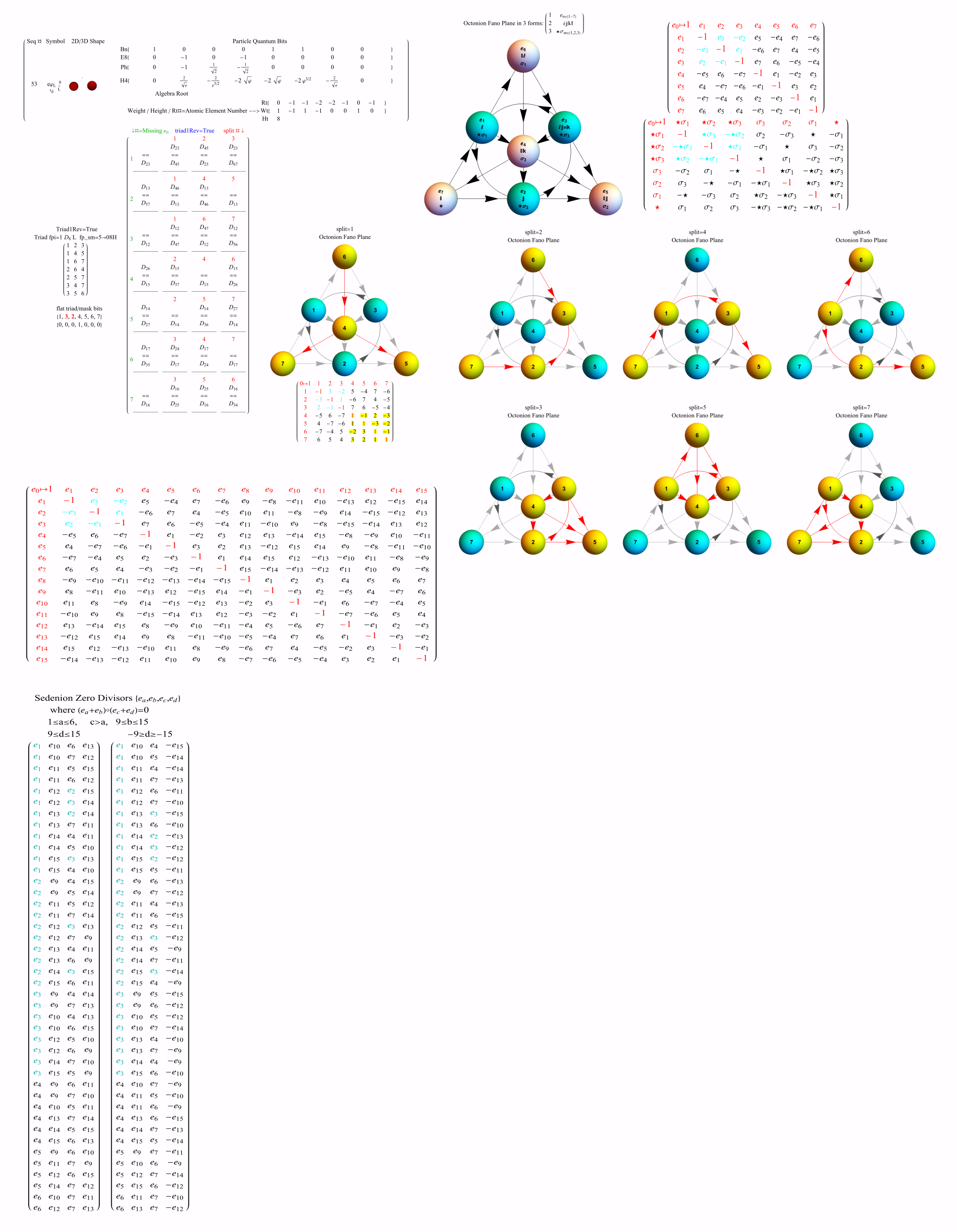
Hypercomplex E8 as it relates to the Sedenions, Trigintaduonions, and beyond

This post will document some work I am doing related to E8, H4, and the hypercomplex forms of algebras and groups. So stay tuned….

Hypercomplex numbers
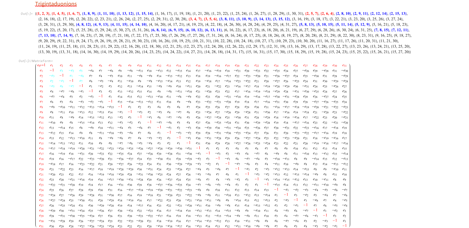
Trigintaduonions derived using repeated Cayley-Dickson doubling of my “Palindromic Octonions” (one of 480 possible) that creates a unique Derivation chart (as shown below). Red are the Octonion triads and Blue are Sedenions.
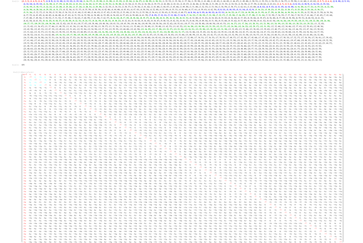
Sexagintaquatronions derived using repeated Cayley-Dickson doubling of my “Palindromic Octonions” (one of 480 possible) that creates a unique Derivation chart (as shown below). Red are the Octonion triads, Blue are Sedenion, and Green are Trigintaduonions.
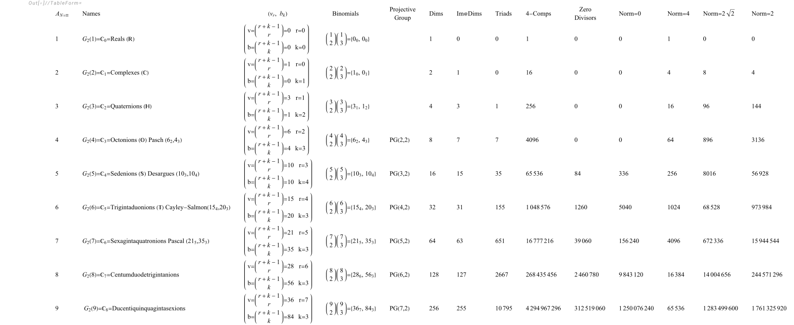
Palindromic Octonions (with 7 split forms) and their Cayley-Dickson generated Sedenions with uniquely symmetric Derivation chart and 84 Zero Divisors