Check out the new demonstrations using free interactive web plugin , .CDF, or .NB (for licensed Mathematica users) and social media integrations for comments, pages and posts.

Check out the new demonstrations using free interactive web plugin , .CDF, or .NB (for licensed Mathematica users) and social media integrations for comments, pages and posts.
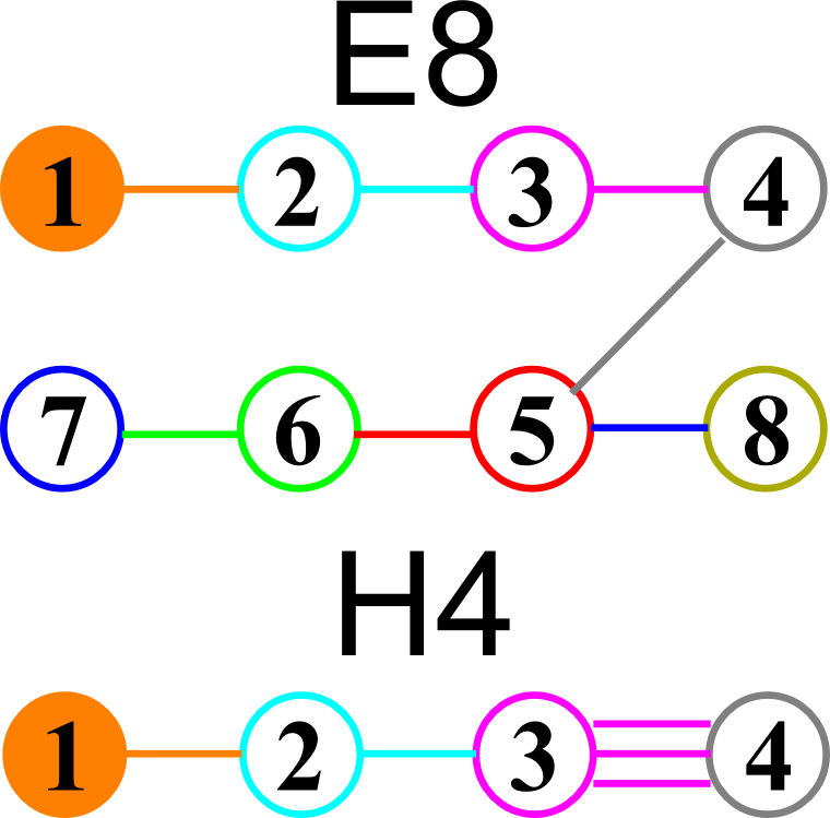
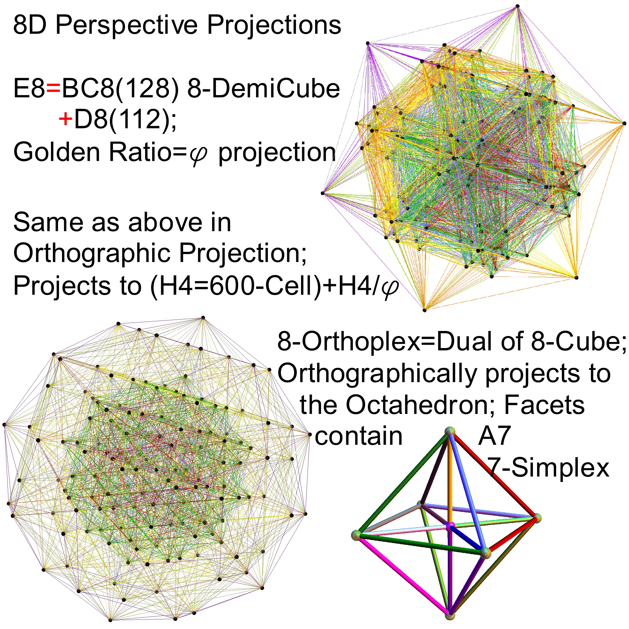
I found the rotation matrix that shows the E8 Dynkin diagram can indeed be folded to H4+H4/φ.
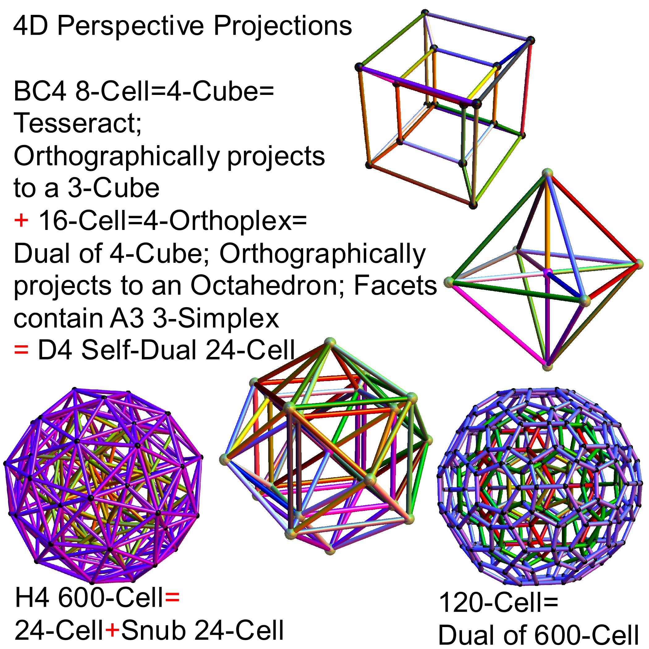
The H4 and its 120 vertices make up the 4D 600 Cell. It is made up of 96 vertices of the Snub 24-Cell and the 24 vertices of the 24-Cell=[16 vertex Tesseract=8-Cell and the 8 vertices of the 4-Orthoplex=16-Cell]).
It can be generated from the 240 split real even E8 vertices using a 4×8 rotation matrix:
x = (1, φ, 0, -1, φ, 0, 0, 0)
y = (φ, 0, 1, φ, 0, -1, 0, 0)
z = (0, 1, φ, 0, -1, φ, 0, 0)
w = (0, 0, 0, 0, 0, 0, φ^2, 1/φ)
where φ=Golden Ratio=(1+Sqrt(5))/2
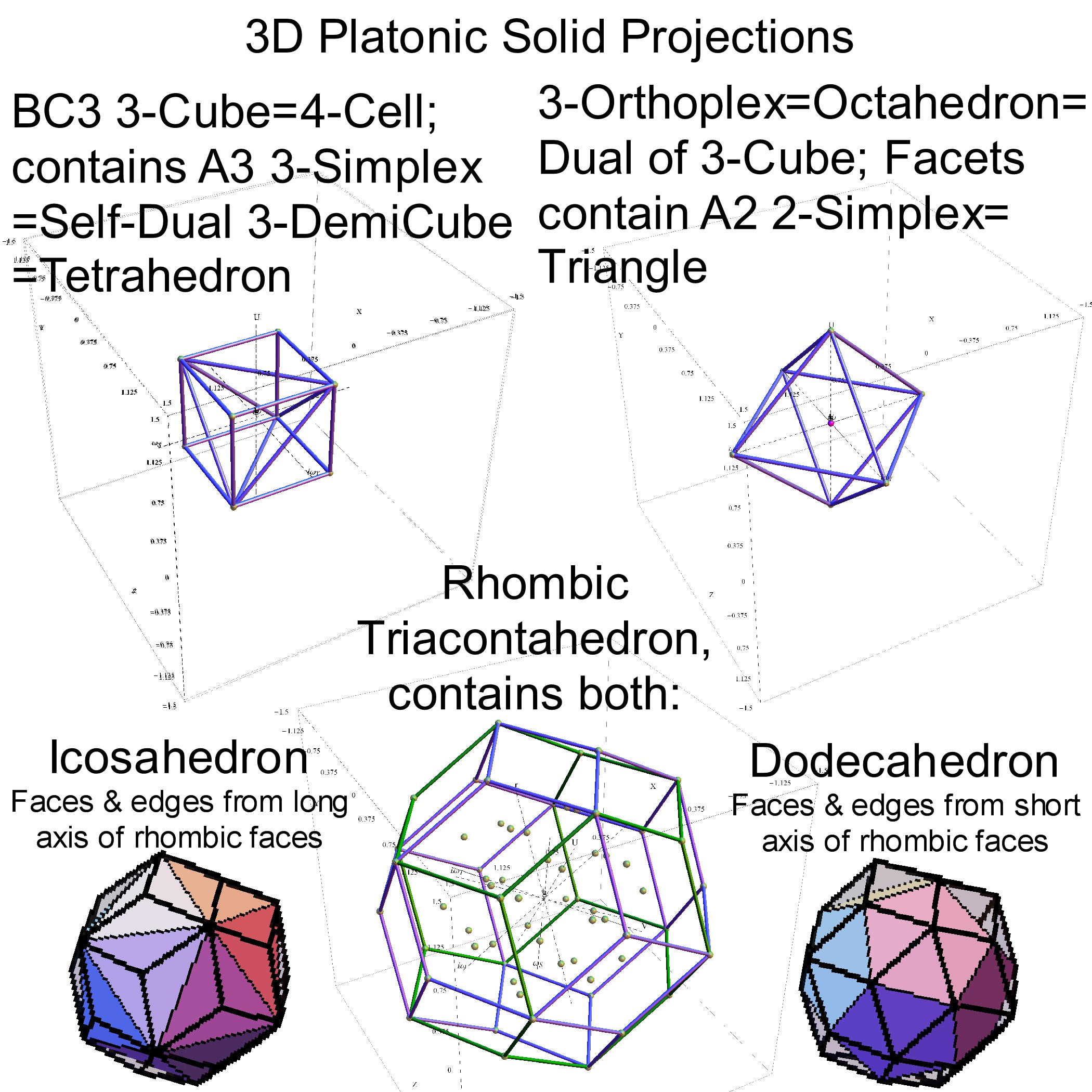
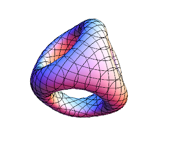
It is also interesting to note that the x, y, and z vectors project to a hull of the 3D Rhombic Triacontrahedron from the 6D 6 cube Hexaract (which then generates the hull of the Dodecahedron and Icosahedron Platonic solids).
Here’s a look at the Dynkin Diagram folding of E8 to H4+H4/φ:
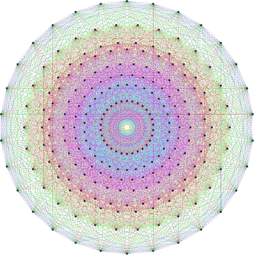
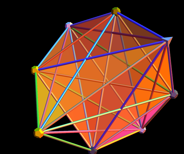
I find in folding from 8D to 4D, that the 6720 edge counts split into two sets of 3360 from E8’s 6720 length Sqrt(2), but the combined edges and vertices recreate the E8 petrie diagram perfectly.
Some visualizations of this in 8D:
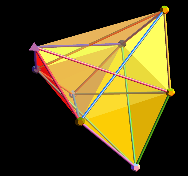
to 4D:
and also showing the Rhombic Triacontrahedron folding from 6D:
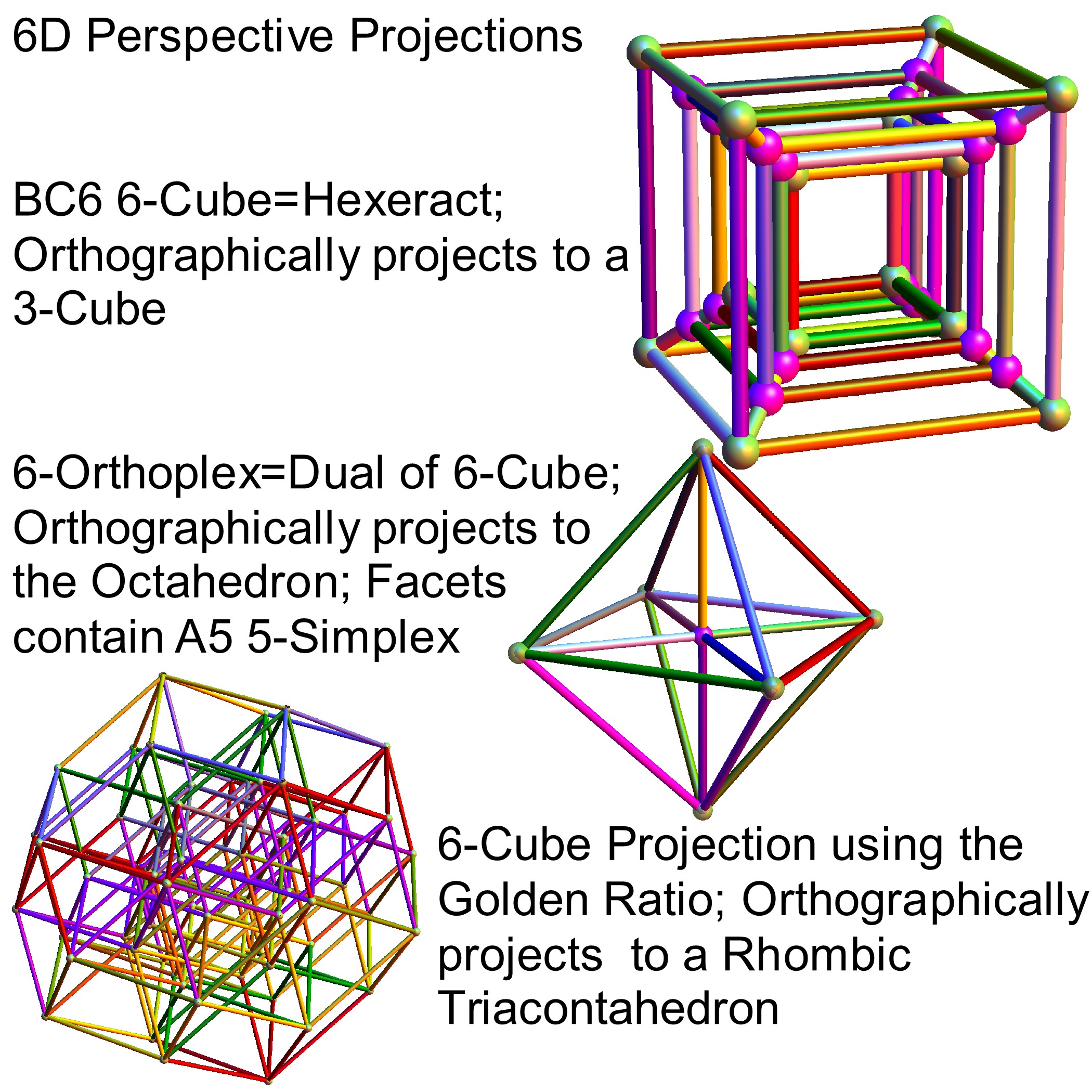
to 3D:
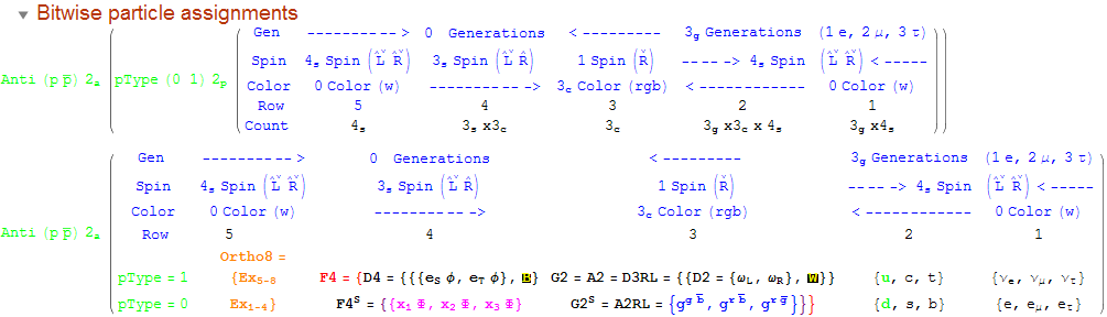
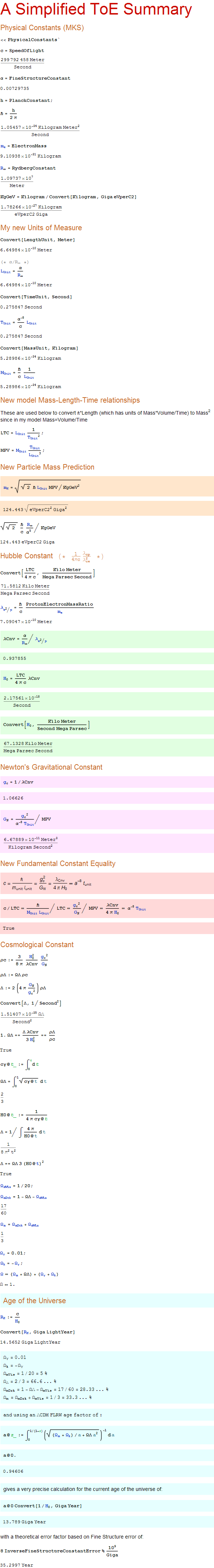
Modified Lisi split real even E8 particle assignment quantum bit patterns:
Assigning a specific mass, length, time, and charge metrics based on new dimensional relationships and the Planck constant (which defines Higgs mass).
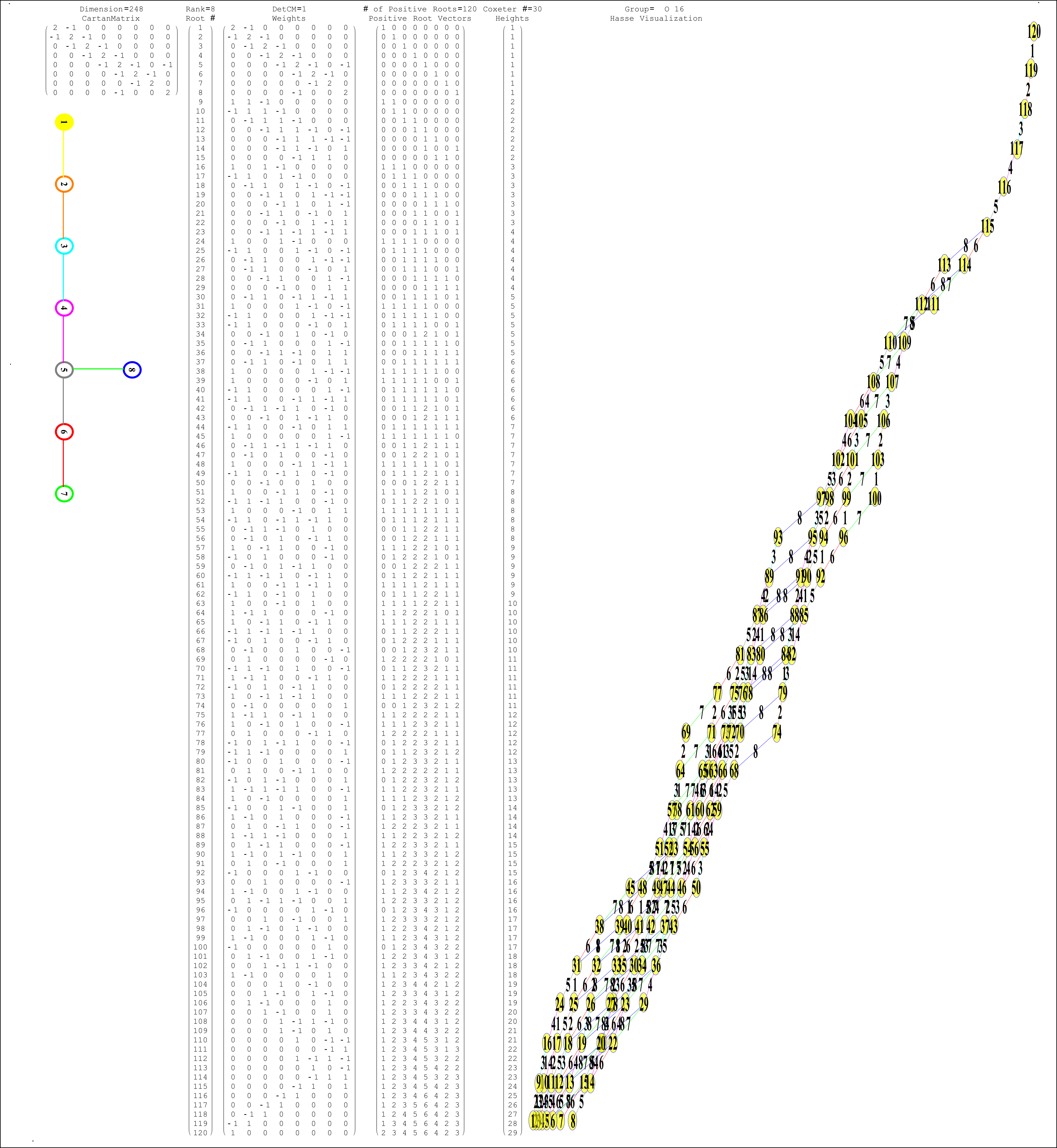
The split real even E8 group used has been determined from this simple root matrix (which gives the Cartan matrix upon dot product with a transpose of itself):
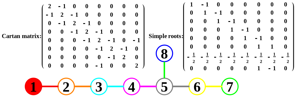
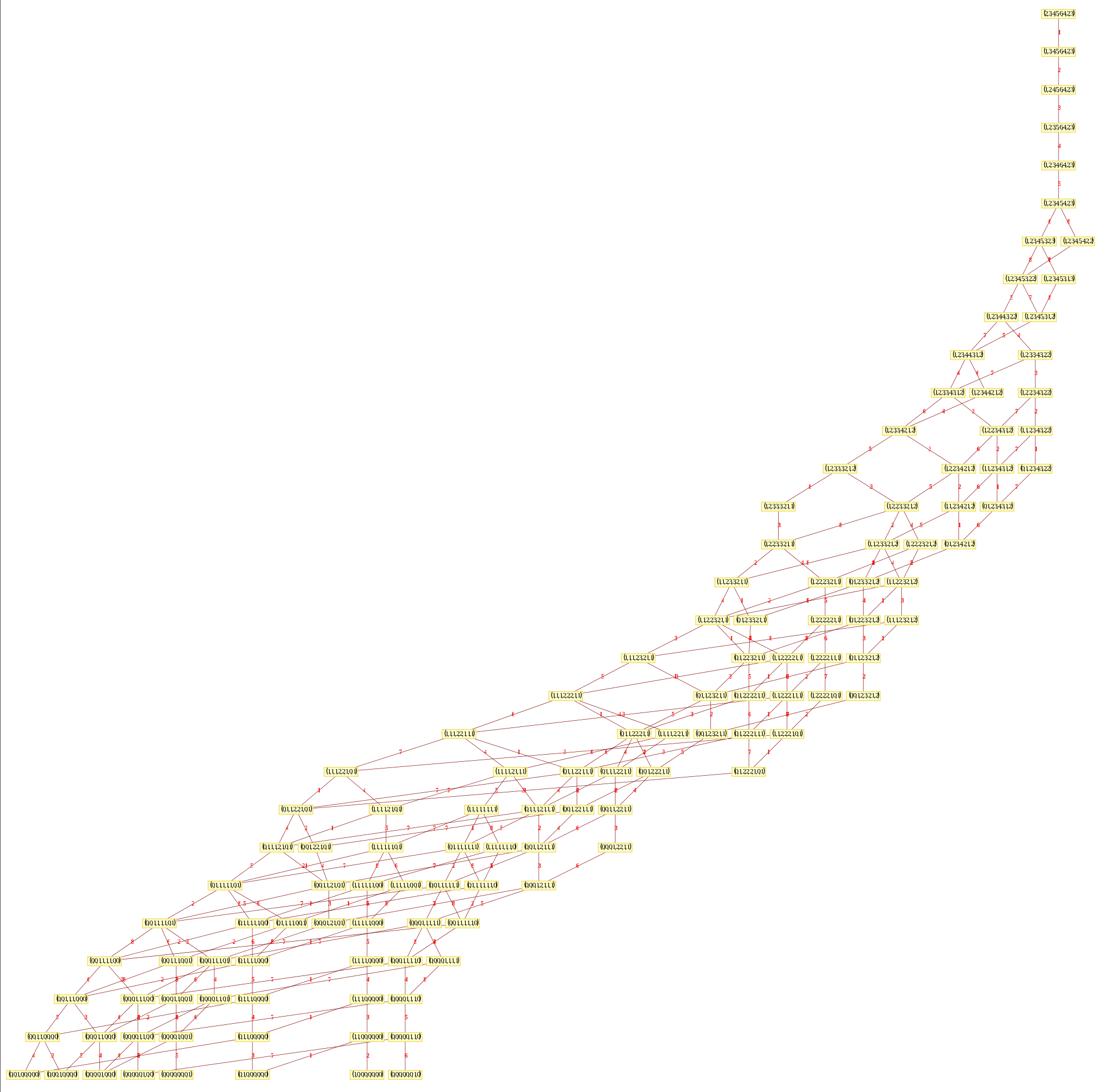
This Dynkin diagram builds the Cartan matrix and determines the root/weight/height with corresponding Hasse diagrams.
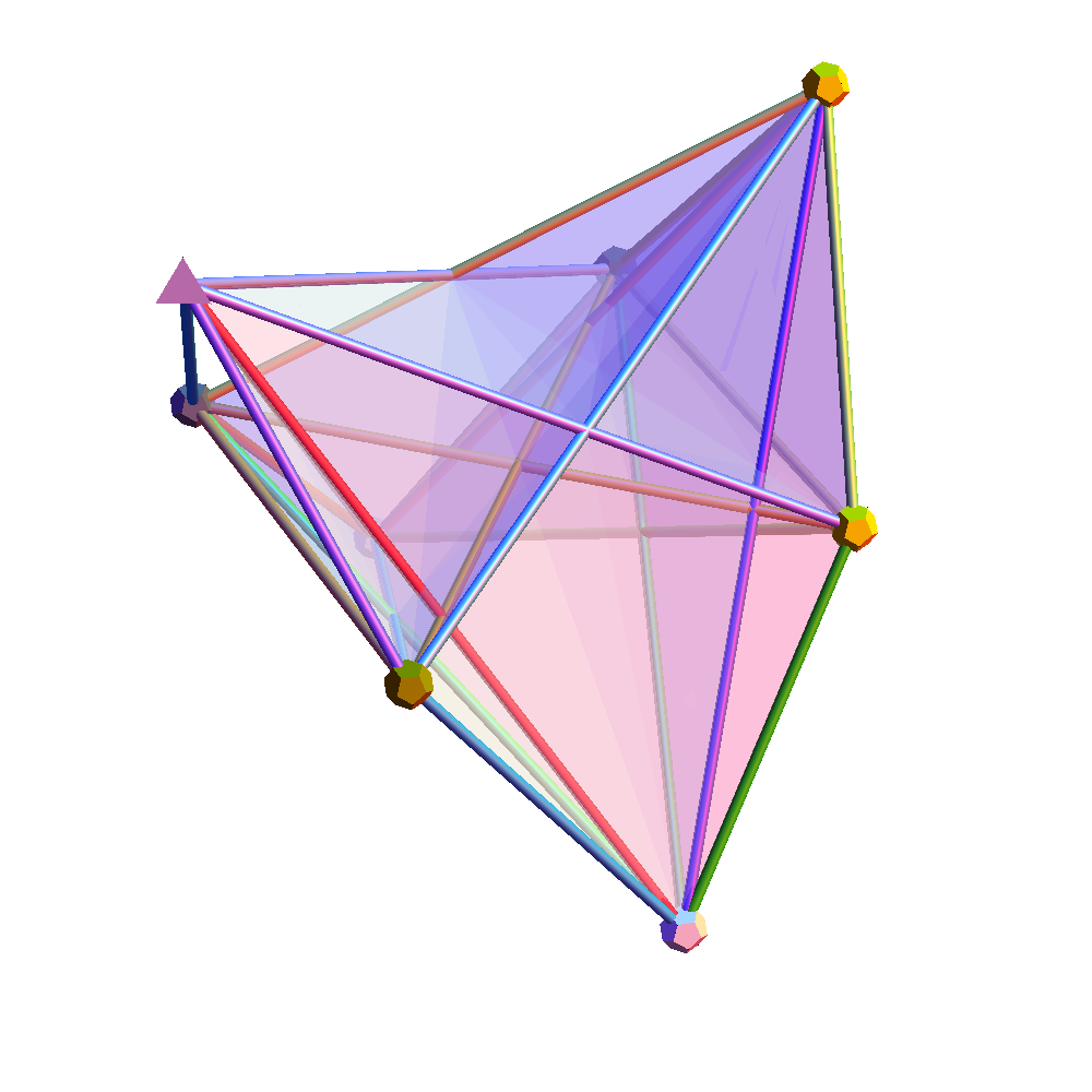
Getting more capability built into ToE_Demonstration.nb where it can now calculate the scattering amplitude by calculating the volume of the projected hull of selected edges in the n-Simplex Amplituhedron (based on a theory by Nima Arkani-Hamed, with some Mathematica code from J. Bourjaily for the positroid diagram). Of course, there is still much work to get this wrapped up…
A few more pics of Positive Grassmannian Amplituhedrons…
This last diagram is obtained using the following amplituhedron0.m as input to the ToE_Demonstration.nb (when using fully licensed Mathematica) as shown below:
* This is an auto generated list from ToE_Demonstration.nb *)
new := {
artPrint=True;
scale=0.1;
cylR=0.018;
range=2.;
pt={-0.3, 0.0, 0.6};
favorite=1;
showAxes=False;
showEdges=True;
showPolySurfaces=True;
eColorPos=False;
dimTrim=5;
ds=6;
pListName=”First8″;
dsName=”nSimplex”;
p3D=” 3D”;
edgeVals={{Sqrt[11/2], 8}, {Sqrt[9/2 – Sqrt[2]], 4}, {Sqrt[9/2 + Sqrt[2]], 4}};
};new;
Positroid Diagrams:
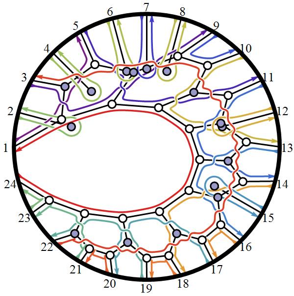
Playing around trying to visualize the latest in the theoretical high energy particle physics (HEP/TH) determining how particle masses might be predicted from geometric principles (based on a theory by Nima Arkani-Hamed, with some Mathematica code from J. Bourjaily for the positroid diagram).
Positive Grassmannian Amplituhedrons
Compare this Mathematica(l) basis to the artistic representation by Andy Gilmore 
Positroid Diagrams:
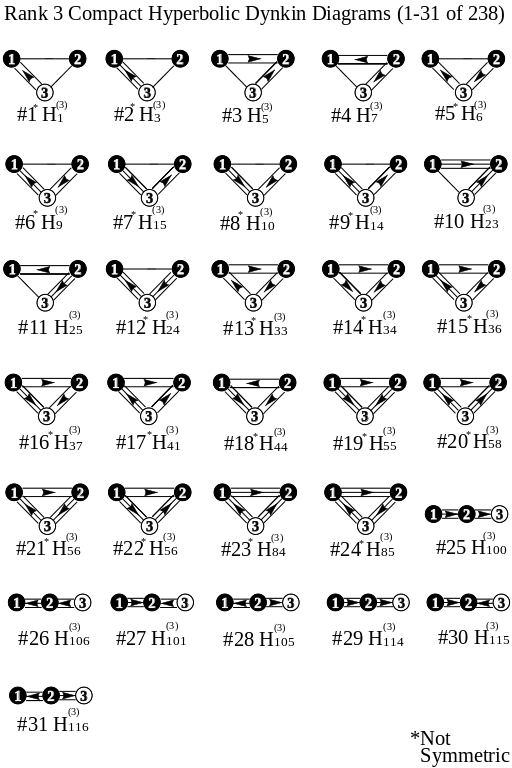
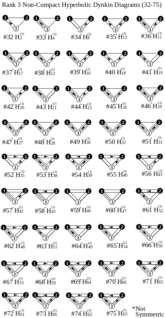
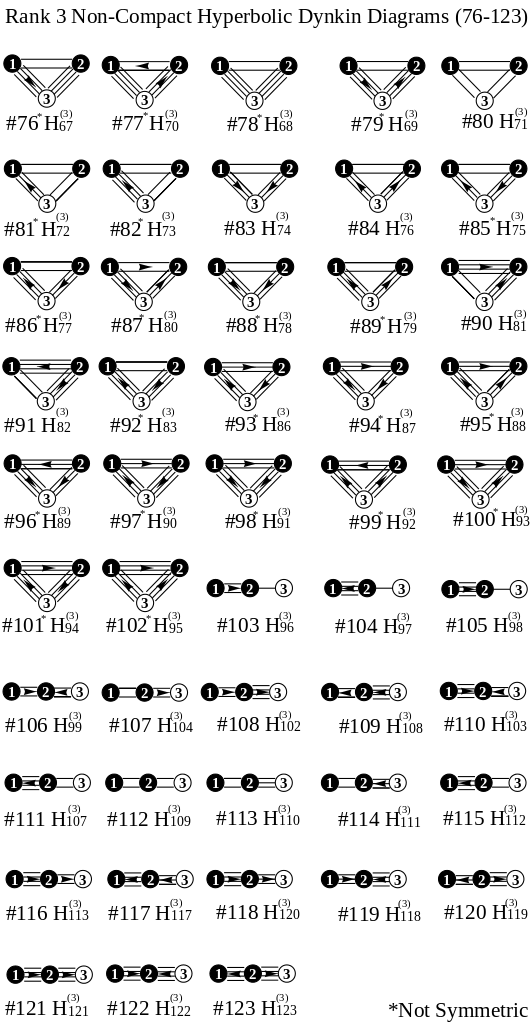
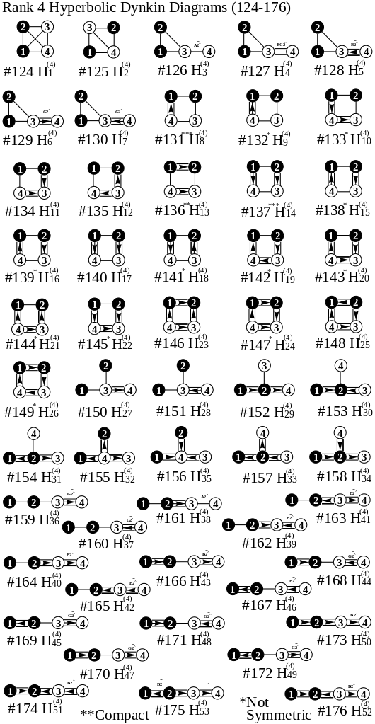
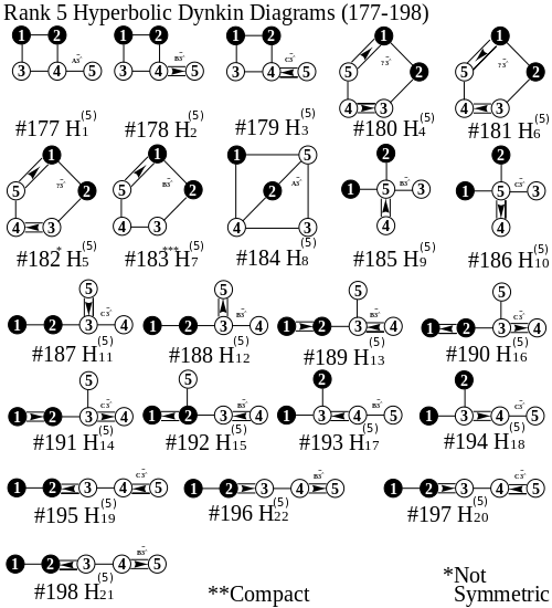
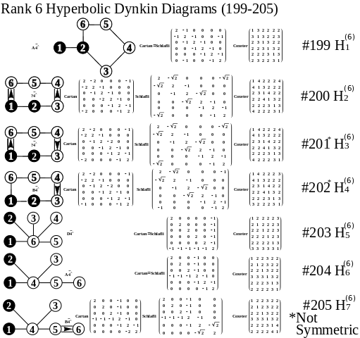
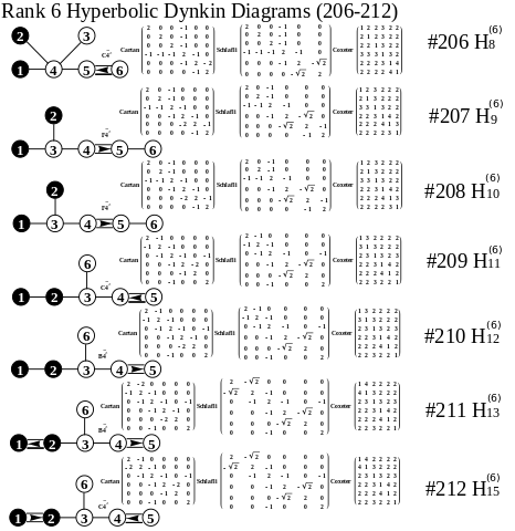
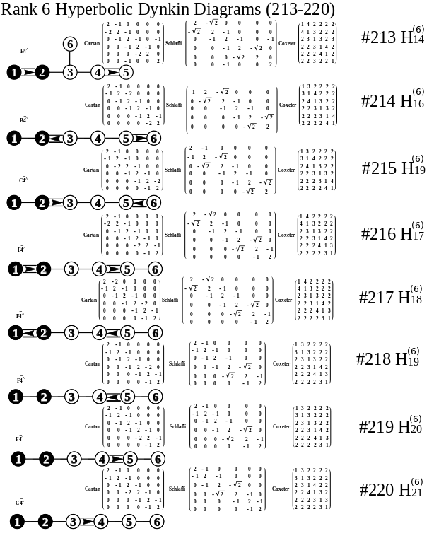
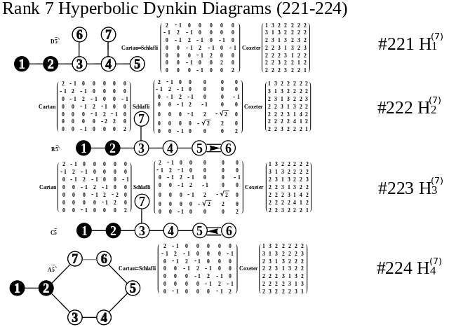
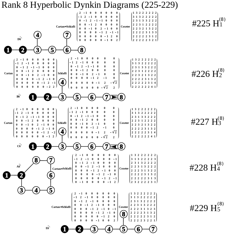
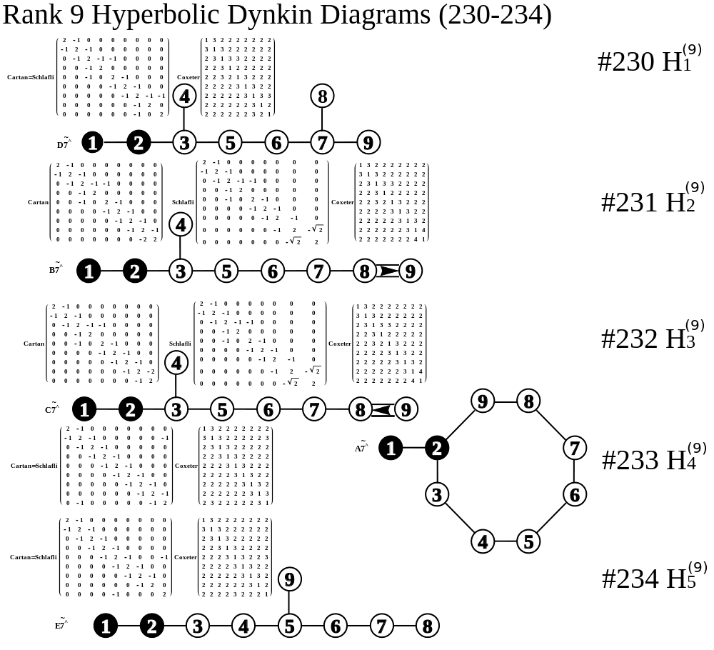
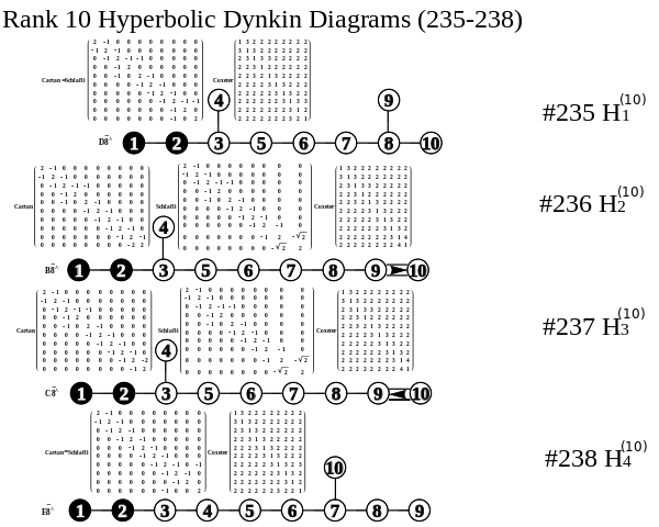
I am pleased to announce the availability of the comprehensive set of 238 Hyperbolic Dynkin diagrams ranks 3 to 10. These are enumerated here. They are constructed interactively using the mouse GUI (or manually through keyboard entry of the node / line tables) from this Mathematica notebook or free CDF player demonstration document or interactive CDF player web page.
All of these demonstrations have now been updated to include the new options on Dynkin diagram creation, including left (vs. right) affine topology recognition, black&white vs. color nodes and edges, and for those with full Mathematica licenses the notebook allows for added Dynkin line types.
The Lie group names are calculated based on the Dynkin topology. The geometric permutation names are calculated (to rank 8) based on the binary pattern of empty and filled nodes. The node and line colors can be used as indicators in Coxeter projections and/or Hasse diagrams.
I’ve updated the .NB, .CDF and interactive demonstrations to include the ability to visualize the split octonions.
With some Mathematica source from Leon Lampret at math.stackexchange.com, I’ve been trying to understand the link between the bitangents of octonions and the Klein Quartic Curves.
Which seems to be closely related to Greg Egan’s wonderful visualization from
http://www.gregegan.net/SCIENCE/KleinQuartic/KleinQuartic.html
Please see this post for updates to these graphs.
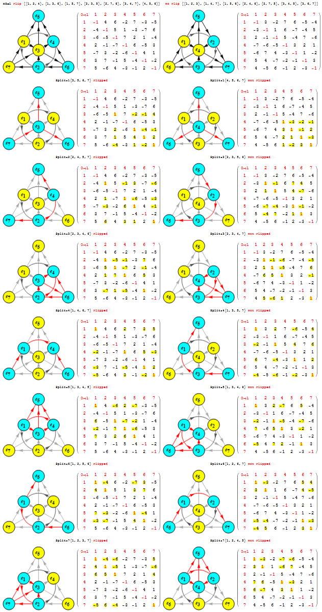
I am pleased to announce the availability of splitFano.pdf, a 321 page pdf file with the 3840=480*8 split octonion permutations (with Fano planes and multiplication tables). These are organized into “flipped” and “non-flipped” pairs associated with the 240 assigned particles to E8 vertices (sorted by Fano plane index or fPi).
There are 7 sets of split octonions for each of the 480 “parent” octonions (each of which is defined by 30 sets of 7 triads and 16 7 bit “sign masks” which reverse the direction of the triad multiplication). The 7 split octonions are identified by selecting a triad. The complement of {1,2,3,4,5,6,7} and the triad list leaves 4 elements which are the rows/colums corresponding to the negated elements in the multiplication table (highlighted with yellow background). The red arrows in the Fano Plane indicate the potential reversal due to this negation that defines the split octonions. The selected triad nodes are yellow, and the other 4 are cyan (25MB).
These allow for the simplification of Maxwell’s four equations which define electromagnetism (aka.light) into a single equation.
I believe this is the only comprehensive presentation of all 3840 Split Fano Planes with their multiplication tables available.
Below is the first page of the comprehensive split octonion list.
Please see Integrated E8, Binary, Octonion for a tutorial that explains the detail of the content of Fano.pdf. It outlines the relationships in the integration of E8 with Octonions, Binary, Particles, NKS, and the Periodic Table of Elements. Other formats are also available (.ppt or .pps and .pdf).