Chaos:
This demonstration combines several demonstrations related to chaos theory, fractals and Navier-Stokes computational fluid dynamics (CFD) as it relates to a theory of a Universe that has a superfluid space-time.
See http://demonstrations.wolfram.com/FiveModeTruncationOfTheNavierStokesEquations/
From Andrew J.Hanson with Additional contributions by Jeff Bryant,
See http://demonstrations.wolfram.com/CalabiYauSpace/
From Yu-Sung Chang,
See http://demonstrations.wolfram.com/ContoursOfAlgebraicSurfaces/
Fano:
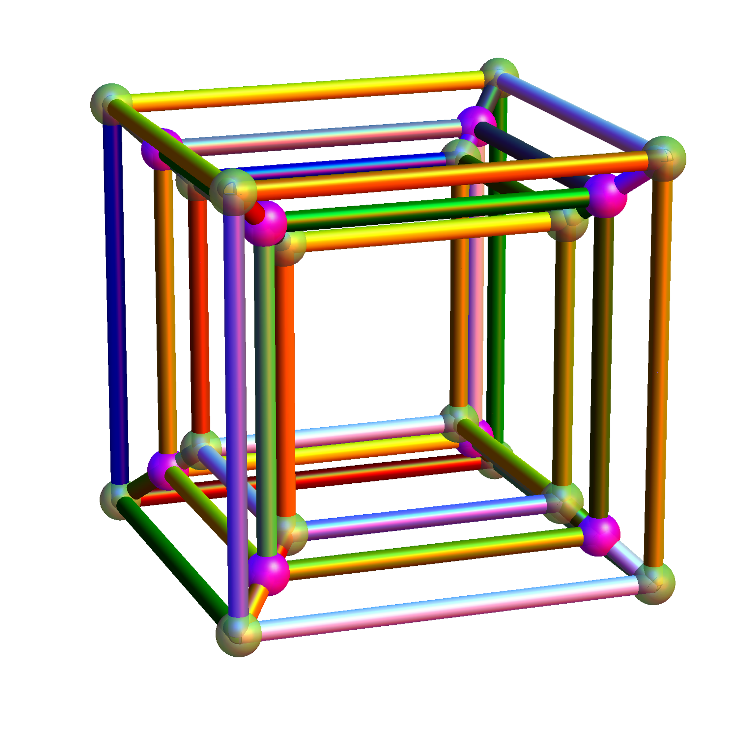
Octonions use a range of 1-7 numbered triplet subsets. A Fano plane is a collection of seven of these triplets (or triads) where no two share two numbers. A Fano plane is a configuration with 30 distinct numberings, when the numbers 1 to 7 (a flattened set of triads) are assigned to the seven points. For each of the 30 distinct numberings, there are eight possible reversals of triplet order, which are identified here as bitwise (hexadecimal) sign masks. These 240=30*8 triplets can also be inverted by inverting the eight sign masks, giving a total of 480 Fano planes. These are visualized here as either a directed 2D graph or a non-directed 3D cubic form. The product of two distinct units equals the third unit, such that the three form immediately connected vertices of the graph.
The octonions can be constructed from quaternions by means of the Cayley-Dickson construction. Like quaternions and the lower-dimensional complex numbers, octonions have one real number (e0=1). Octonions have seven imaginary units e1-e7, or in IJKL format {I,J,K=IJ,L,IL,JL,KL=IJL} whose multiplication tables can be encoded using the Fano plane mnemonic, shown here in both numeric and symbolic form.
For any three octonions a, b, and c, the associator is (a*b)*c – a*(b*c). The associator measures the non-associativity of those three octonions. Select triples of octonionic units to compute their associator. Observe that their associator vanishes on immediately connected triples of octonionic units. Such triples, together with the unit element, form the quaternionic sub-algebras of octonions.
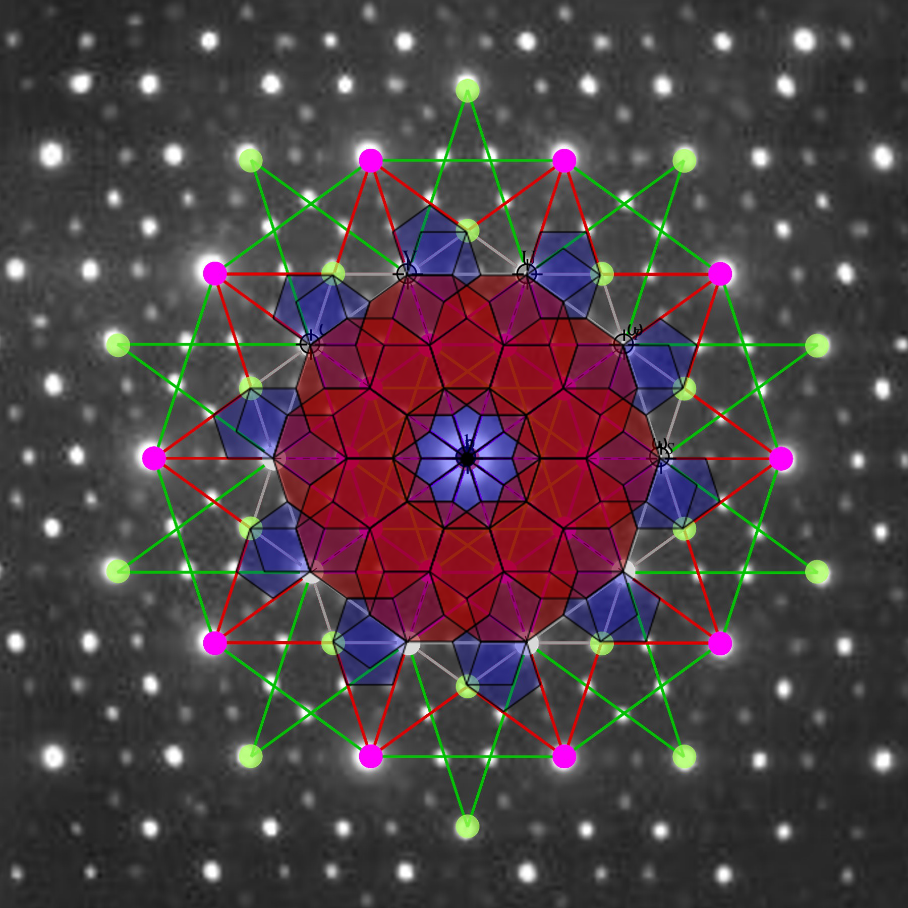
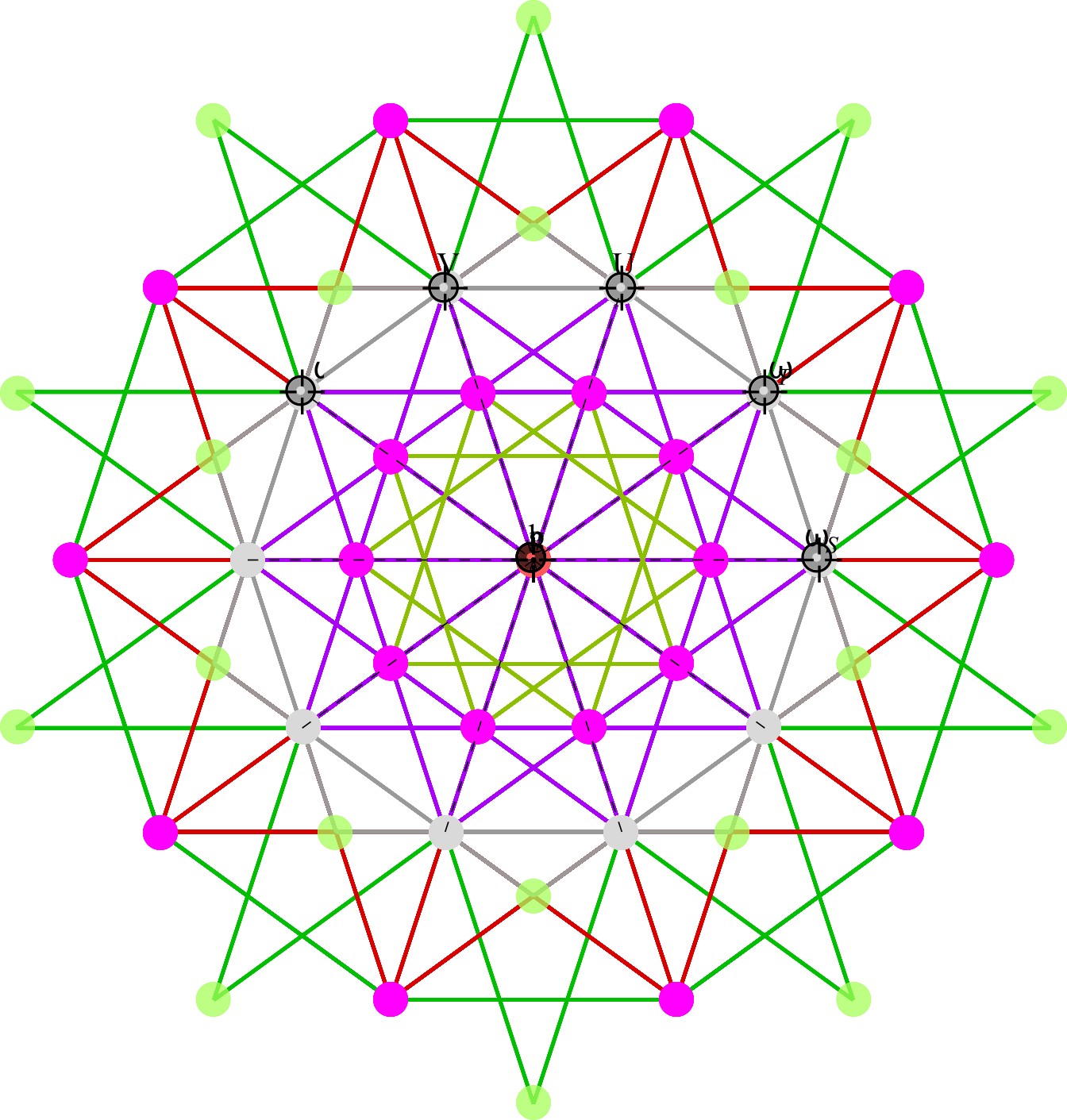
The odd-4 graph is constructed by taking the 35 triplets that share no values. The graph is the odd-4 graph (black edge lines). If a 1-7 point Fano plane is removed from the odd-4 graph, the result is the Coxeter graph (cyan edge lines). If connections to the fifteen Fano planes of a single color are added instead, the result is the Hoffman-Singleton graph (yellow edge lines). The Fano plane index (fPi) driven by fp_gen and fp_color determines the type (cyan or yellow) of graph.
Select any of the 480 permutations for the Fano basis using the same bit-wise quantum particle selections (described in the “Particle” section below, with the addition of the “flip” check-box to select the second E8 linked octonion for the particle). Red or blue numbers in the flattened triads indicate it is one of 240 E8 related permutations needing those colored node positions flipped (or reversed) to create a proper Fano plane from it. Blue indicates it is a member of the 128-vertex C8 subgroup of E8 and red for subgroup D8 with 112 vertices. Node colors are changed from cyan to yellow for button bar selected associator dimensions {n1,n2,n3}. A selection to view the symbolic multiplication tables in IJKL form is also included. Octonion math examples are shown below the numeric and symbolic multiplication tables.
Each new selection of the 480 different bases changes the octonion multiply and commutator results and verifies the conjugate, norm, and division results are the same. This verifies proper octonion operation as shown in the octonion math examples.
The construction of the 480 octonion sets of 7 triples uses converted C source code from Donald Chesley of Davidson Laboratories, Stevens Institute of Technology.
The list of 30 Fano planes (made up of sets of 7 quaternion triads) can be determined algorithmically by brute force (checking each of the 35 possible unique triples against the 21 possible unique pairs and finding the 30 sets of 7 that don’t share more than one number).
The 16 sign mask (sm) sets can also then be algorithmically determined for each index into 30 sets of Fano plane quaternion triads (by taking each of the 30 Fano planes and brute force checking which of the 128=2^7 sign reversal bit patterns keep the associator=0). Each sign reversal constitutes an arrow direction reversal in the Fano plane mnemonic.
It turns out that all of the 128=2^7 possible bit patterns for reversing the Fano plane arrows is used. These are grouped into 2 sets of 64 with an “anti” (or 0< ->1 bit reversal) operation. The 64 are found to be grouped into 8 sets of 8 which get associated (or indexed) with the 30 Fano planes. The tally of these associations between the 8 sign mask sets and the 30 Fano plane sets is {{1,2},{2,2},{3,7},{4,3},{5,3},{6,7},{7,3},{8,3}}. That is, there are 4 of the 8 that associate with 3 Fano planes each. There are 2 of the 8 that associate with 7 Fano planes and 2 that associate with 2 of them.
A split of the 30 triad sets into 15=7+8 (or D8+C8) provides the indicator on where to assign the “excluded” permutations. They get the 0 color and 0 generation assignment – the same logic applied to the excluded E8 vertices or particles. It becomes trivial to apply a naive sequential assignment of 30 Fano planes into two sets of 7/8 assigned to the 4 bits associated with generation and color in the Lisi model.
The binary patterns for the 8 sign mask groups are easily seen and can also be constructed (rather than brute force determined) using right/left symmetry patterns. Interestingly, this construction uses a Clifford algebra Cl(0,8) primitive idempotent e{2,3,5,8} (and its inverse e{1,4,6,7}) as a base. These sets are assigned (R)ight and (L)eft based on the pattern of adding Reverse@Range@3 to 1 (or subtracting Range@3 from 8) respectively. More interestingly, these are also used in assigning the octonions to the E8 particle assignments – specifically, they index to the 4 spins (up/down, left/right) with the set assigned by the pType (neutrino/electron lepton or up/down quark split). These two groups of 4 are also used to index the 15=7+8 (or D8+C8) split associated with generation and color bits. This is a common pattern between the split of octonions into the Cayley-Dickson quaternions (the first 4 a-p & spin bits of the first quaternion e0-e3 and the second 4 color-generation bits of the second quaternion e4-e7).
The Fano plane indices also “pair up” when assigning the 480 octonion permutations into the 240 E8 permutations with D8Pairs={{1,2},{4,7},{8,10},{15,16},{17,19},{23,24},{25,26}} and C8Pairs={{3,5},{6,9},{11,12},{13,14},{18,20},{21,22},{27,29},{28,30}}. The pairs are always found together in the E8 particle assignment as “flipped” and “non-flpped” Fano planes (except the last of the C8 Pairs {28,30}, which have an anomalous flip pattern associated with the 3rd generation blue quarks).
To reach the doubling of the 512=480+32 “excluded” octonion permutations, I added what I call a 9th “flip” bit parameter. This correlates well with A Zee’s approach to grand unification using a 9D SO(18) group theory. It turns out that the pattern required for flipping works in unison with the a and p bits in a binary logic relationship. As the demonstration clearly shows, the p bit flips the two sets of four sm bits. This is the key to a eureka moment where I created the notion of a 3rd spin type out of the pType bit (in/out or z-x or yaw intrinsic rotation or spin). Also note: Charge-Parity-Time (CPT) conservation law (symmetry) considerations also strongly link these a, p, and spin bits.
The binary logic relationship with the “flip” bit and the sm bits clearly create two 4 bit quaternion sets. The first quaternion is the anti(e0=1 Real) bit combined with 3 spin bits {e1,e2,e3} or {I,J,K=IJ}. The second quaternion is 2 generation bits {e4,e5} or {L,IL} combined with 2 color bits {e6,e7} or {JL,KL=IJL}. While this double set of quaternions was already obvious to me from the E8 construction (noted in http://theoryofeverything.org/TOE/JGM/DynkinParticleReductions.cdf), it was good to confirm it with octonion integration! It seems that this pair of quaternions could be visualized as Hopf Fibrations on 7-manifolds (see http://www.nilesjohnson.net/seven-manifolds.html for an excellent review of this).
A recent addition allows for the visualization of split octonions. The 3840=480*8 split octonion permutations with Fano planes and multiplication tables are now available.
There are 7 sets of split octonions for each of the 480 “parent” octonions. The 7 split octonions are identified by selecting a triad. The complement of {1,2,3,4,5,6,7} and the selected triad list leaves 4 elements which are the rows/colums corresponding to the negated elements in the multiplication table (highlighted with yellow background). The red arrows in the Fano Plane indicate the potential reversal due to this negation that defines the split octonions.
This demonstration now also includes the ability to generate the sedenions from octonions through the application of the Cayley-Dickson doubling procedure. As in the animated Fano Cube, the sedenion display includes the generation of an animated Fano Tesseract mnemonic visualization which steps through highlighting the vertices/edges of the 34 sedenion triads.
These allow for the simplification of Maxwell’s four equations which define electromagnetism (aka.light) into a single equation.
See http://en.wikipedia.org/wiki/Split-octonion
It correlates well with my theory relating time to octonions, charge to quaternions and 3-space to complex (imaginary) numbers. This idea also validates the dimensional considerations that started me down this path 15 years ago (documented in http://theoryofeverything.org/TOE/JGM/ToE.pdf).
This demonstration combines and extends Wolfram demonstrations from Wolfram’s Ed Pegg Jr. (Odd4GraphFanoPlanesAndTheCoxeterGraph) and Oleksandr Pavlik (OctonionsAndTheFanoPlaneMnemonic).
Dynkin:
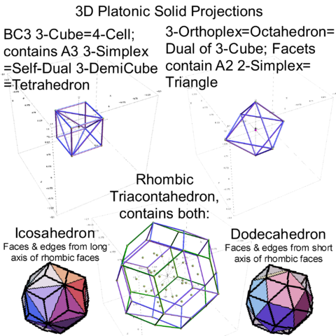
This demonstration lets you create and manipulate multiple Dynkin and Coxeter-Dynkin diagrams with some ability for topological pattern recognition of known Simple Lie Groups (up to rank 8 ) and its designated type, including finite, affine, hyperbolic, and very extended.
You can use the drop down “Dynkin diagrams” to get various diagrams and geometric permutations.
It also provides for manipulating, recognizing, and naming of the 2^rank (binary) Coxter-Dynkin geometric permutations on uniform polyhedron and their Wythoff construction operator naming. These permutations are indicated by filled nodes. When more than one diagram is created, they can be interpreted as a geometric Cartesian product, such as a DuoPrism.
The Cartan matrix which defines the Lie algebra (along with the Coxeter, and Schlafli matrices) are calculated directly from the last diagram entered. If there are more than one diagrams, all with the same rank, the diagram matrices are dotted together.
The main window is a clickable pane.
Clicking more than 1.5 cells away from all nodes creates a new diagram.
Clicking less than 1.5 cells away from all nodes creates a node and a single line to its nearest neighboring node.
Clicking on a node in the last diagram created toggles the node fill on/off and changes the geometric permutation (unless it is an already filled node that is adjacent to an unlinked node, which implies the creation of an affine loop).
Clicking on a line between nodes in the last diagram created toggles the symmetry angle and/or the directionality between its nodes.
Please note that when more than one diagram is in the clickable pane, only the last diagram is active. Clicking on previous diagrams will create a new overlapping diagram.
For better Dynkin diagram topology recognition, select the affine level early and create the linear (A type diagram) nodes before any off-linear nodes (for D and E diagrams).
For more information on Dynkin Diagrams, see http://en.wikipedia.org/wiki/Dynkin_diagram
For more information on Simple Lie Groups, see http://en.wikipedia.org/wiki/Simple_Lie_group
For more information on Coxeter-Dynkin Diagrams, see http://en.wikipedia.org/wiki/Coxeter-Dynkin_diagram
For more information on Coxter-Dynkin geometric permutations on uniform polyhedron and their Wythoff construction operator naming, see http://en.wikipedia.org/wiki/Uniform_polyhedron
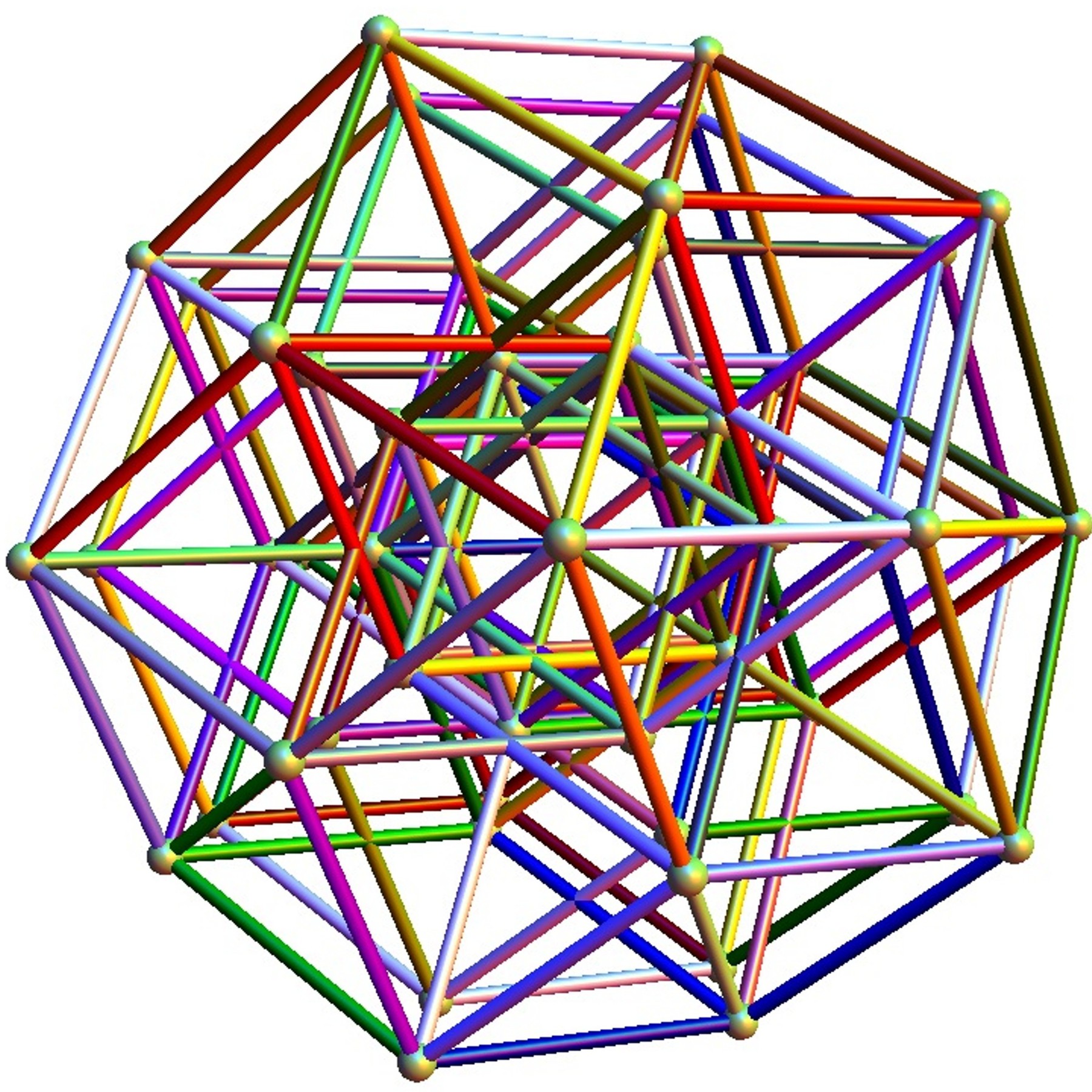
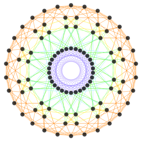
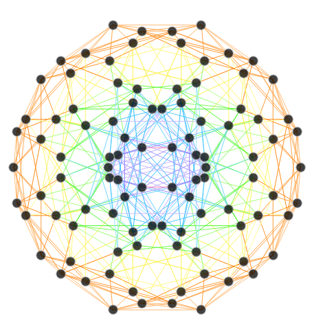
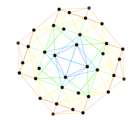
E8:
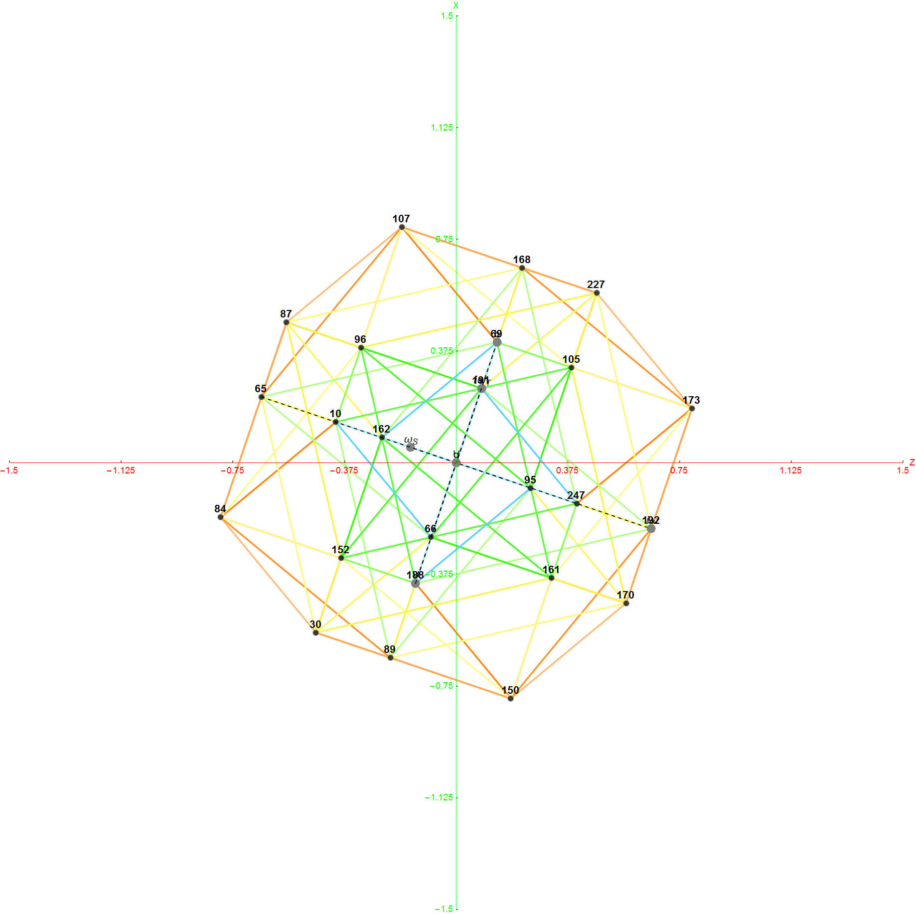
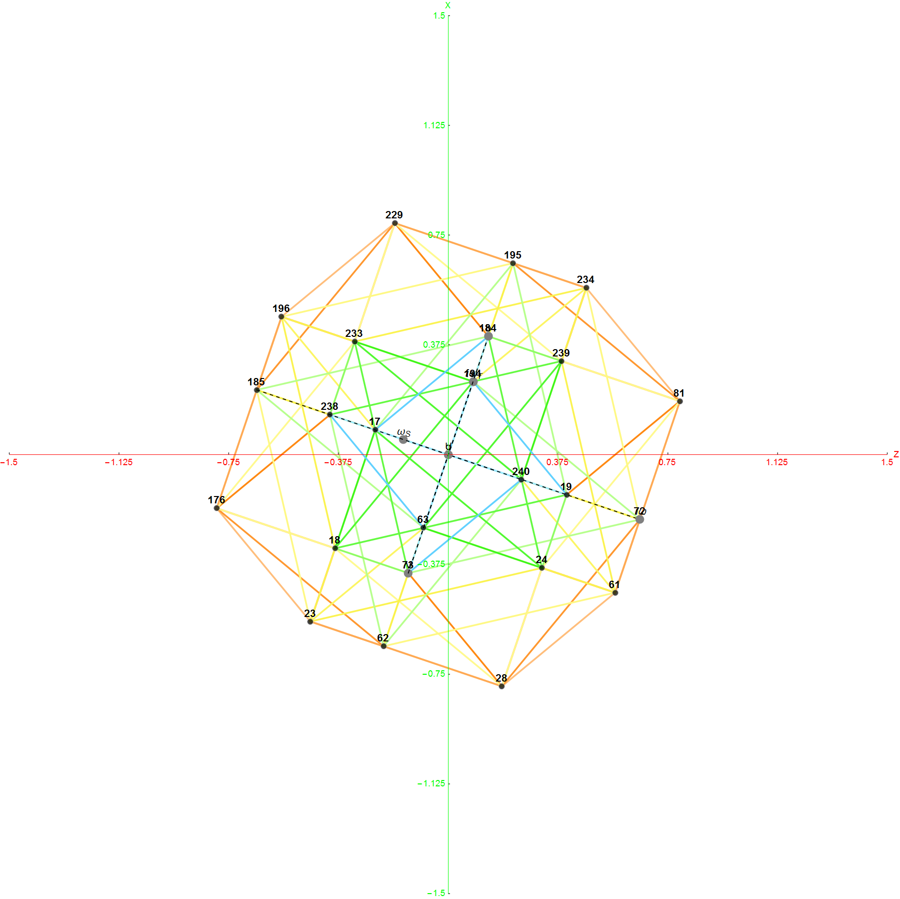
The first drop down list provides for the selection of Coxeter (and other) projection symmetries. Most names indicate Simple Lie groups. The Bn and Cn groups are the same as the ones for Dn+1. (e.g. the menu label “D+1=BC3” applies to D4, B3, and C3 simple Lie algebras or groups and will be projected to their Petrie projection with the basis vectors associated with this menu selection). The next set of projections indicate the number of perimeter vertices in parenthesis. The PASCAL# projections display the number of vertices in a column which is has the same number as that numbers row of the Pascal triangle.
The next two menus provide “Favorites” that are preset combinations of over 50 variables to produce beautiful projections of E8 and its subgroups. Their short names attempt to indicate what is in the resulting image. For example, the references to “n Cube Pascal” in menu 2 refers to a projection that creates columns of vertices (as in the PASCAL# in the Coxeter projection menu). The references to Petrie refer to the corresponding Petrie projection of that n dimensional cube. Favorite names using the word “binary” imply it uses a purely binary data set from the Pascal triangle instead of SRE E8.
The counts of selected vertices, edges, triality lines, and clicked vertex edge lines are shown.
The check boxes select major elements of what gets displayed in the output window:
* axes selects whether to show the 8 axes (and the frame bounding box)
* edges selects whether to show the edges between each vertex (subsets of edge lengths is selected in the HMI pane 8)
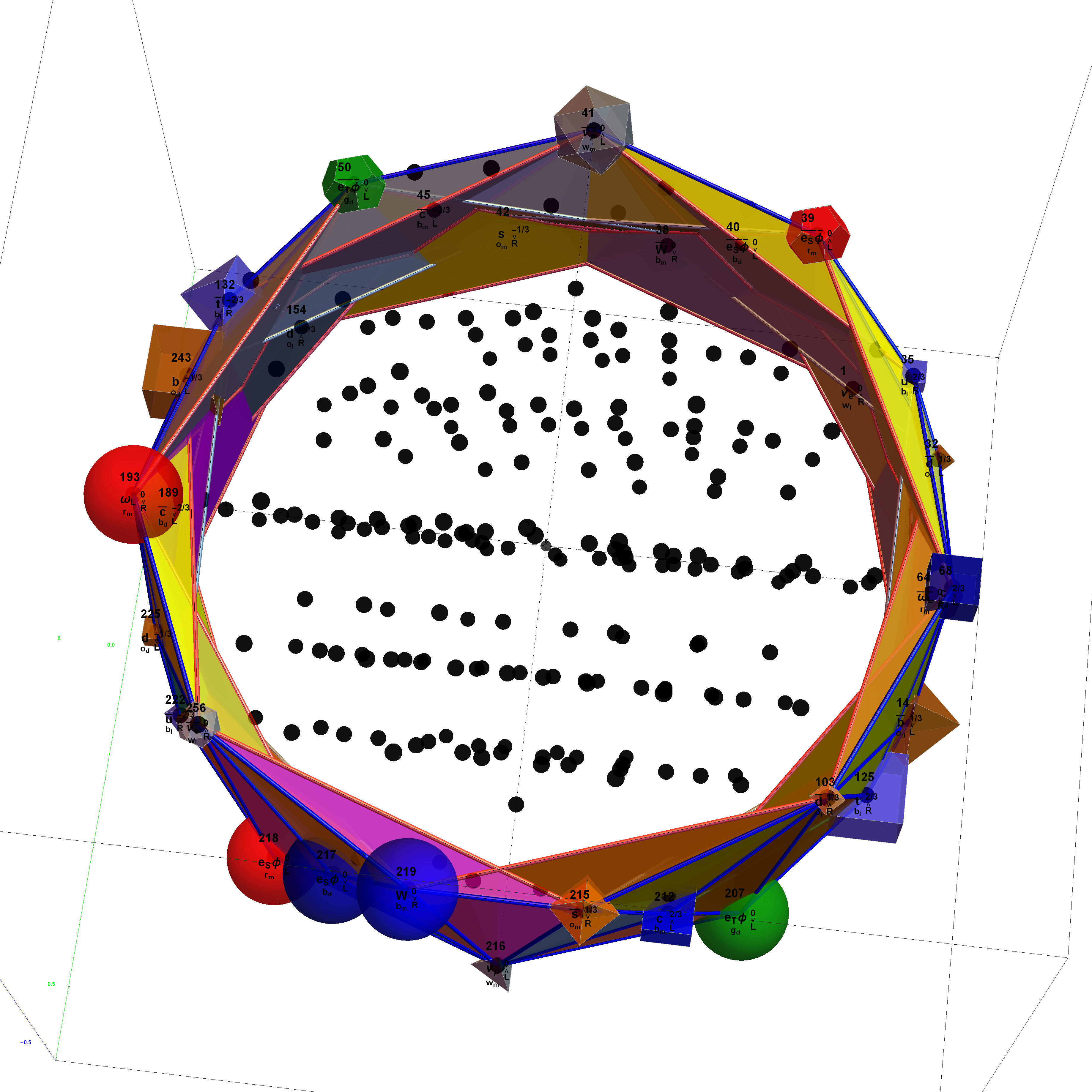
* physics shows the assigned physics particle shape/color/size (vs. dots)
* labels shows the particle labels
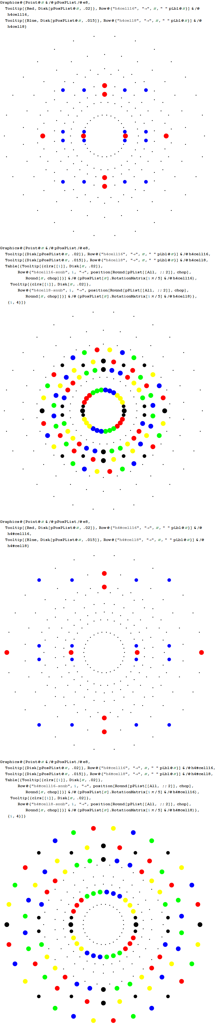
* dimLocs checkbox is used to activate the dimension locators in 2D (deactivates particle interactions).
Checking the “axes locator” box forces it into 2D mode with axes shown. Instead of being a clickable pane, you can now drag the locators on the basis vectors to show new projections on the horizontal and vertical 2D plane using “H” and “V”. The controls to change the azimuthal (Z) basis vector are not available for manipulation in this Demonstration.
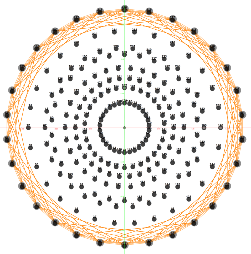
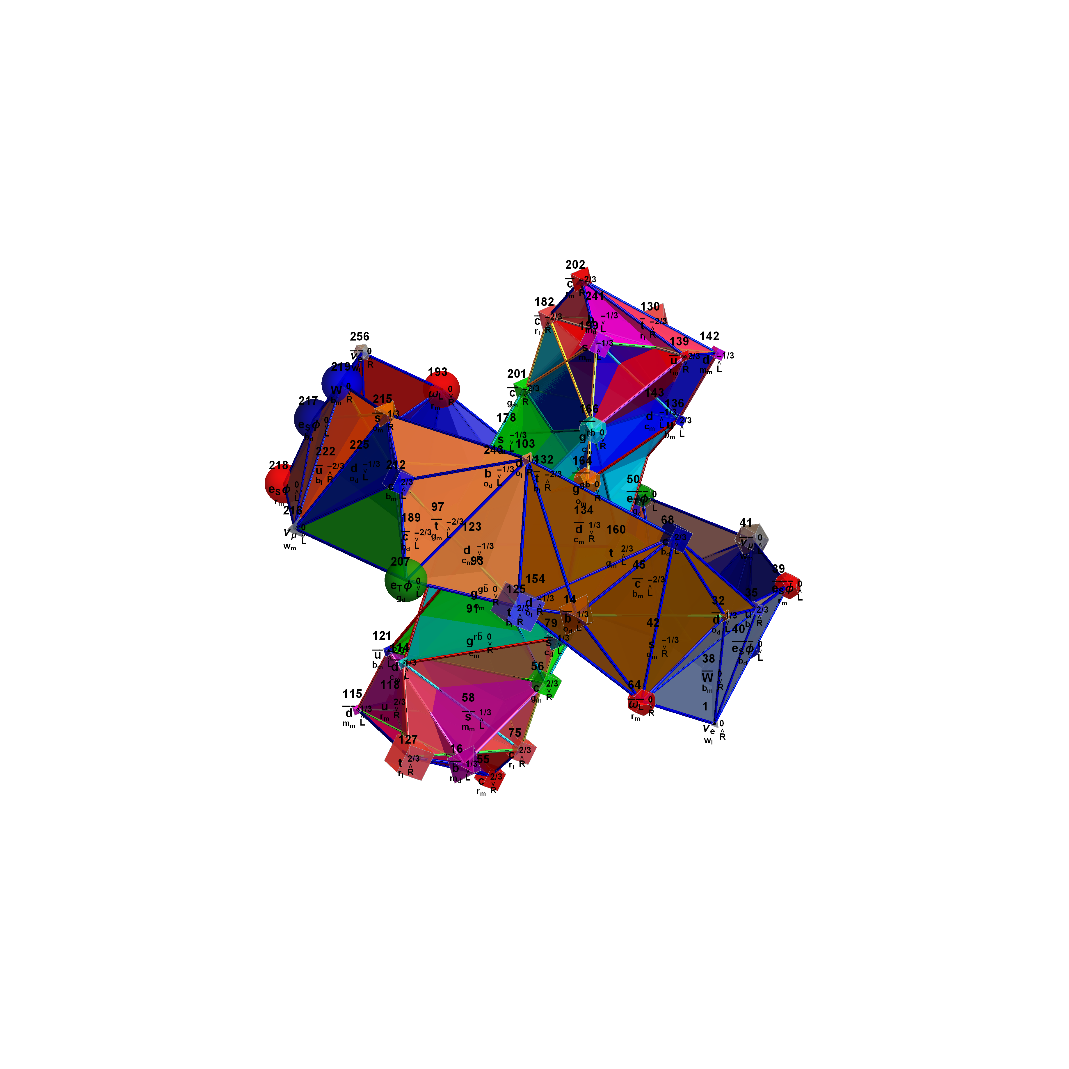
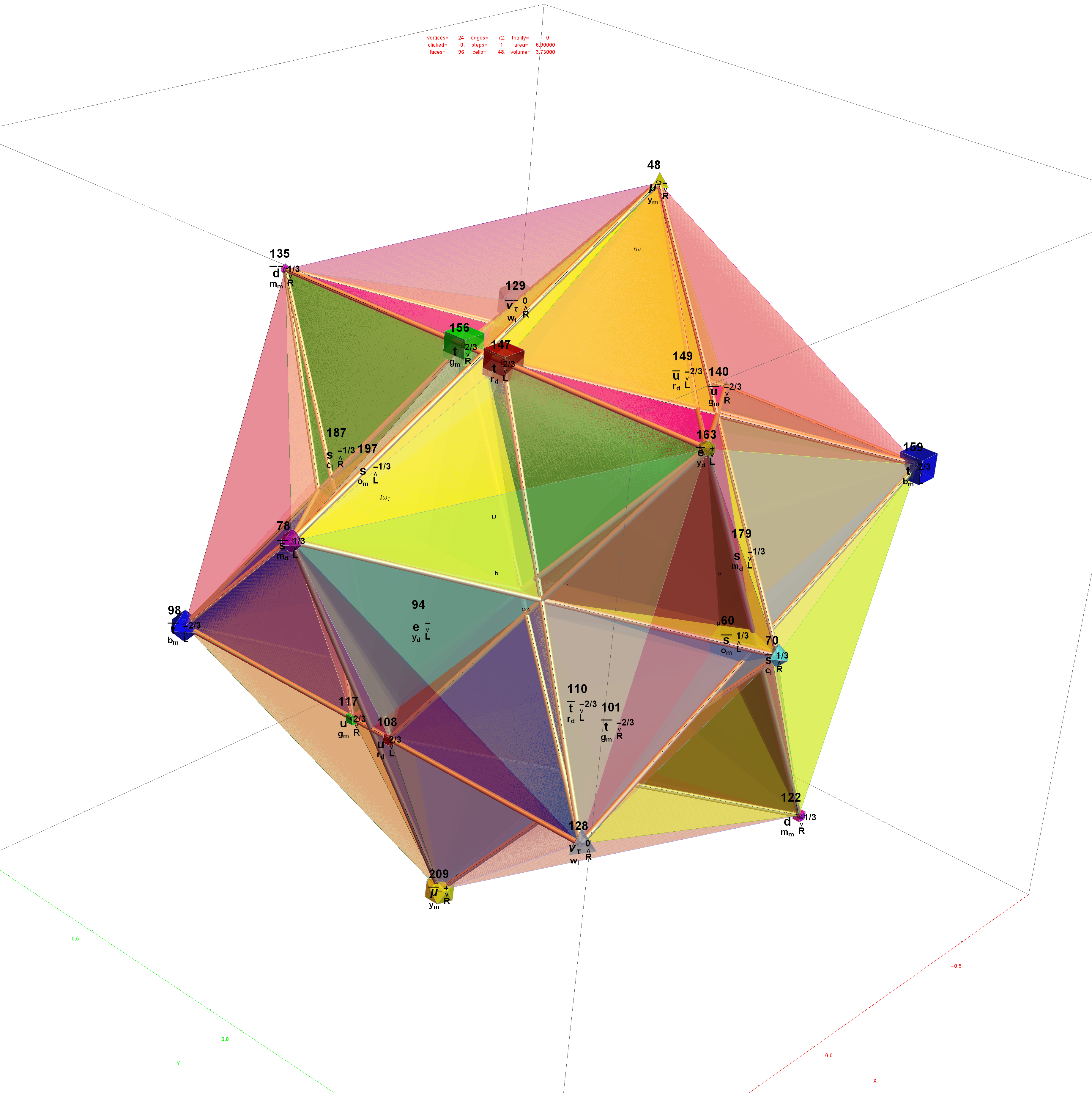
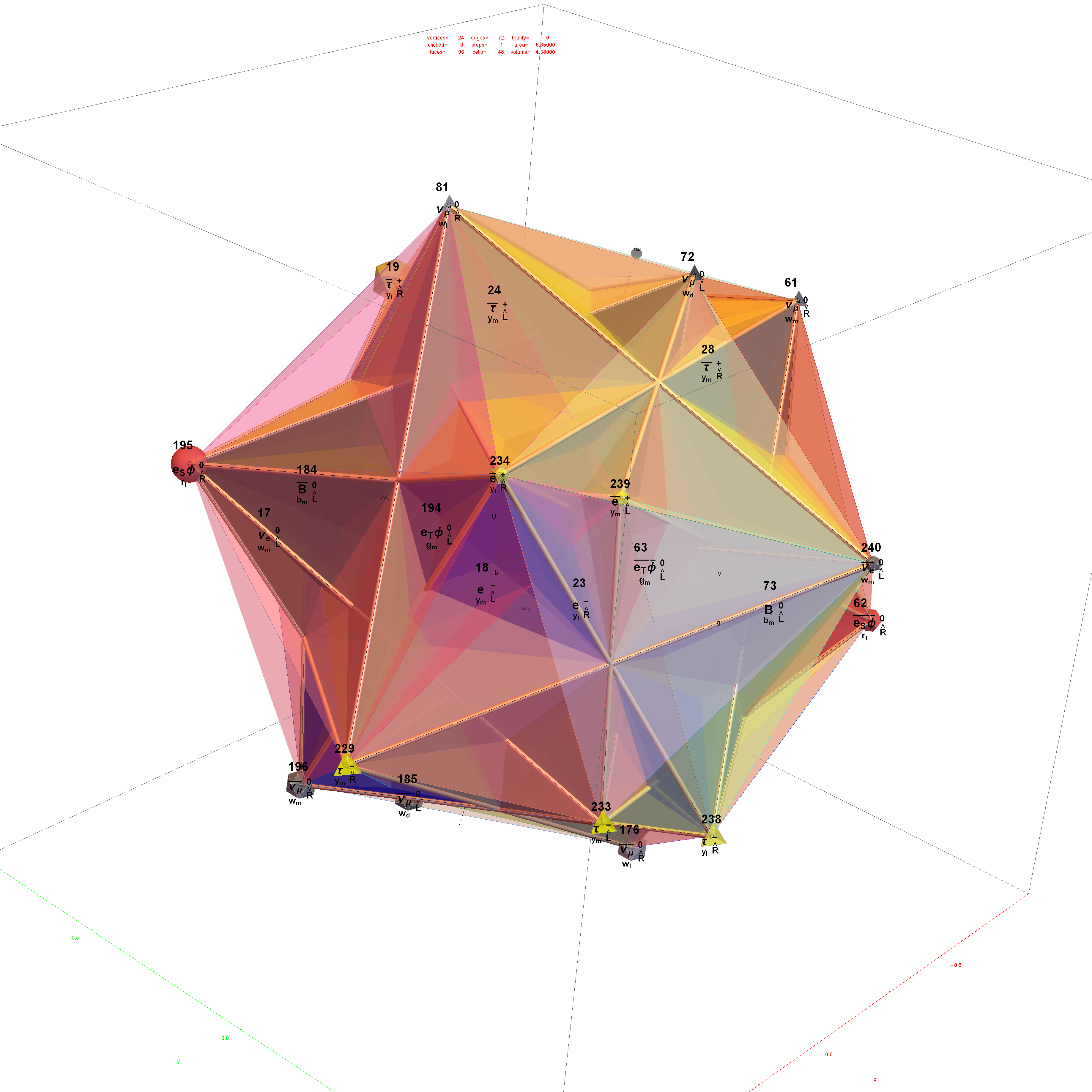
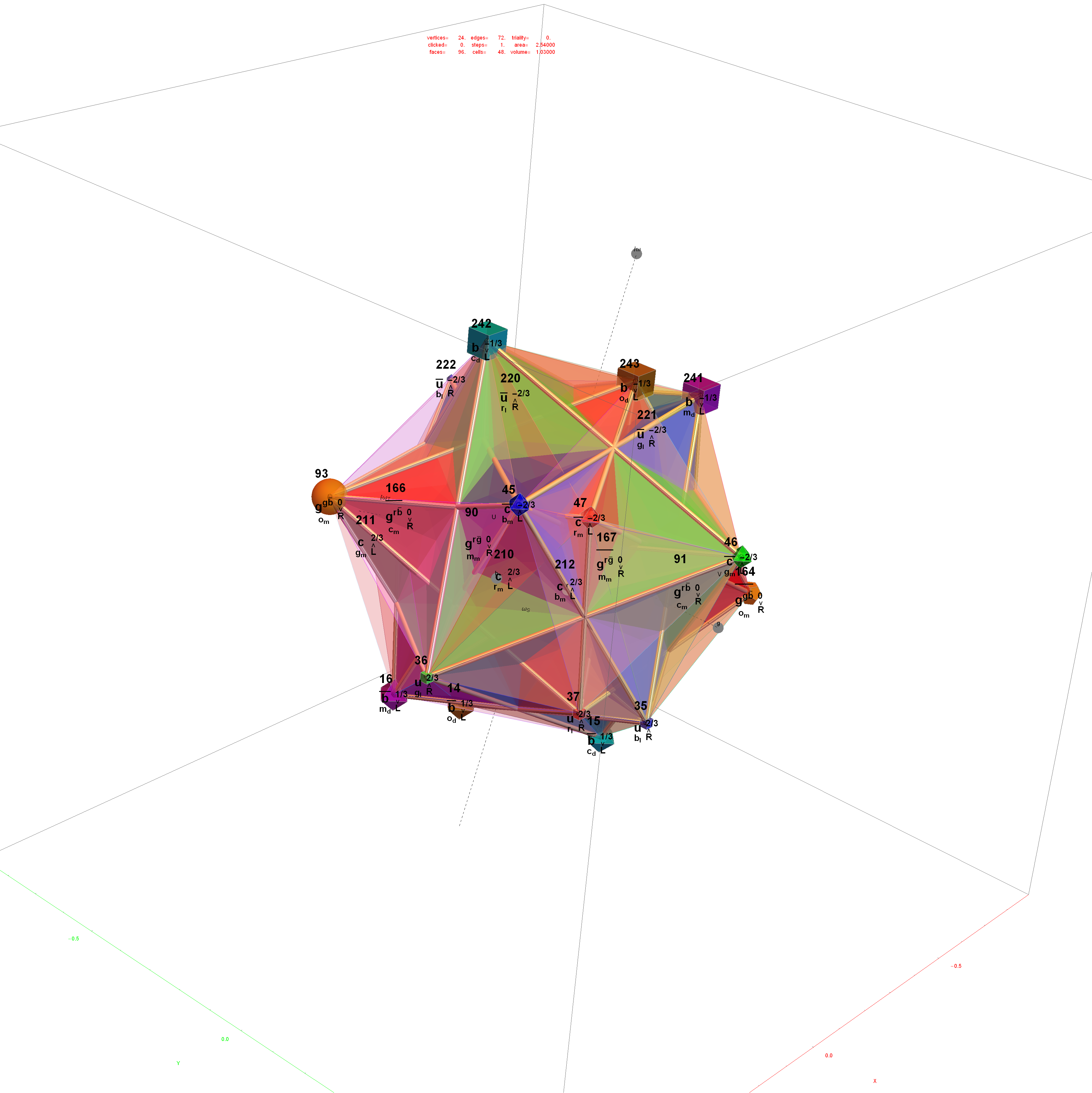
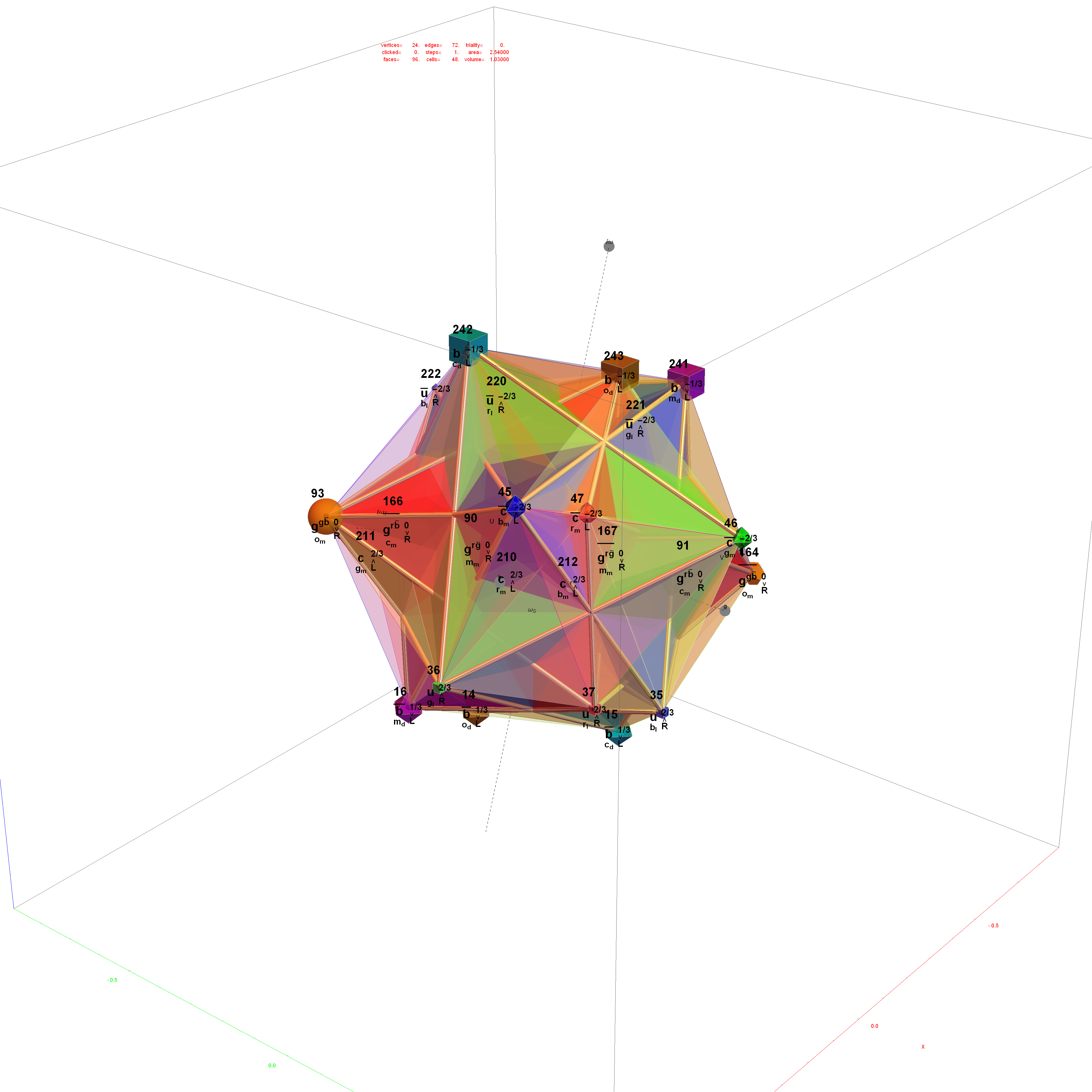
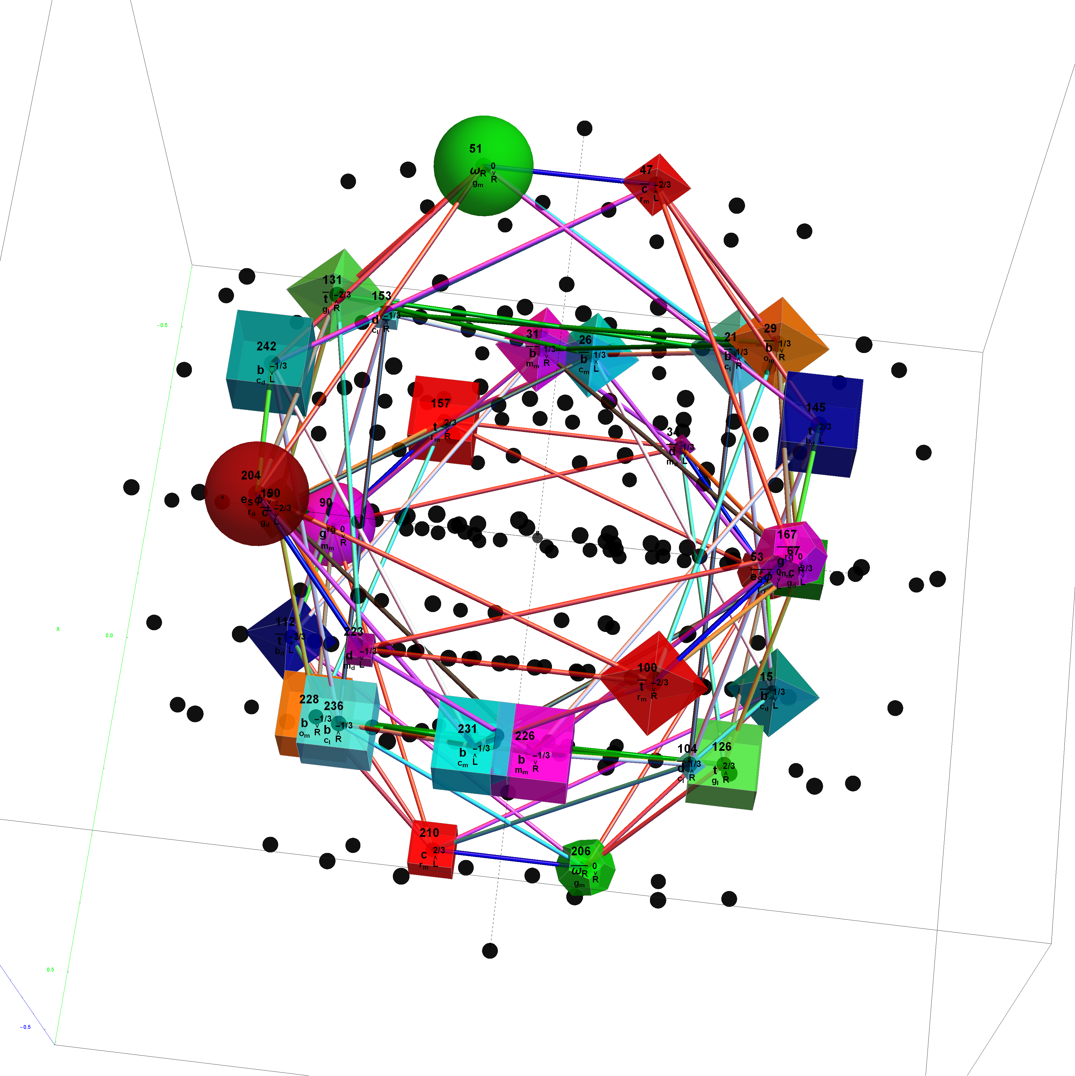
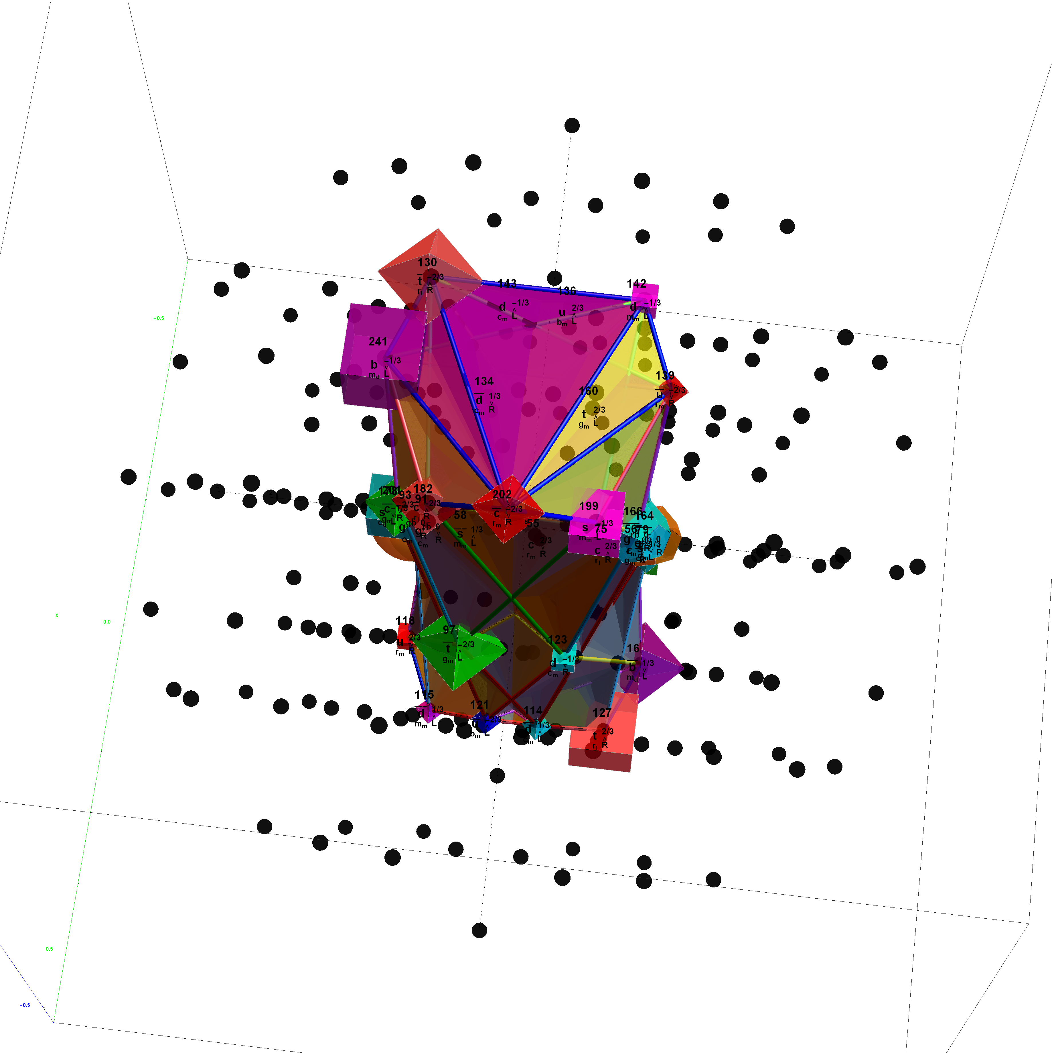
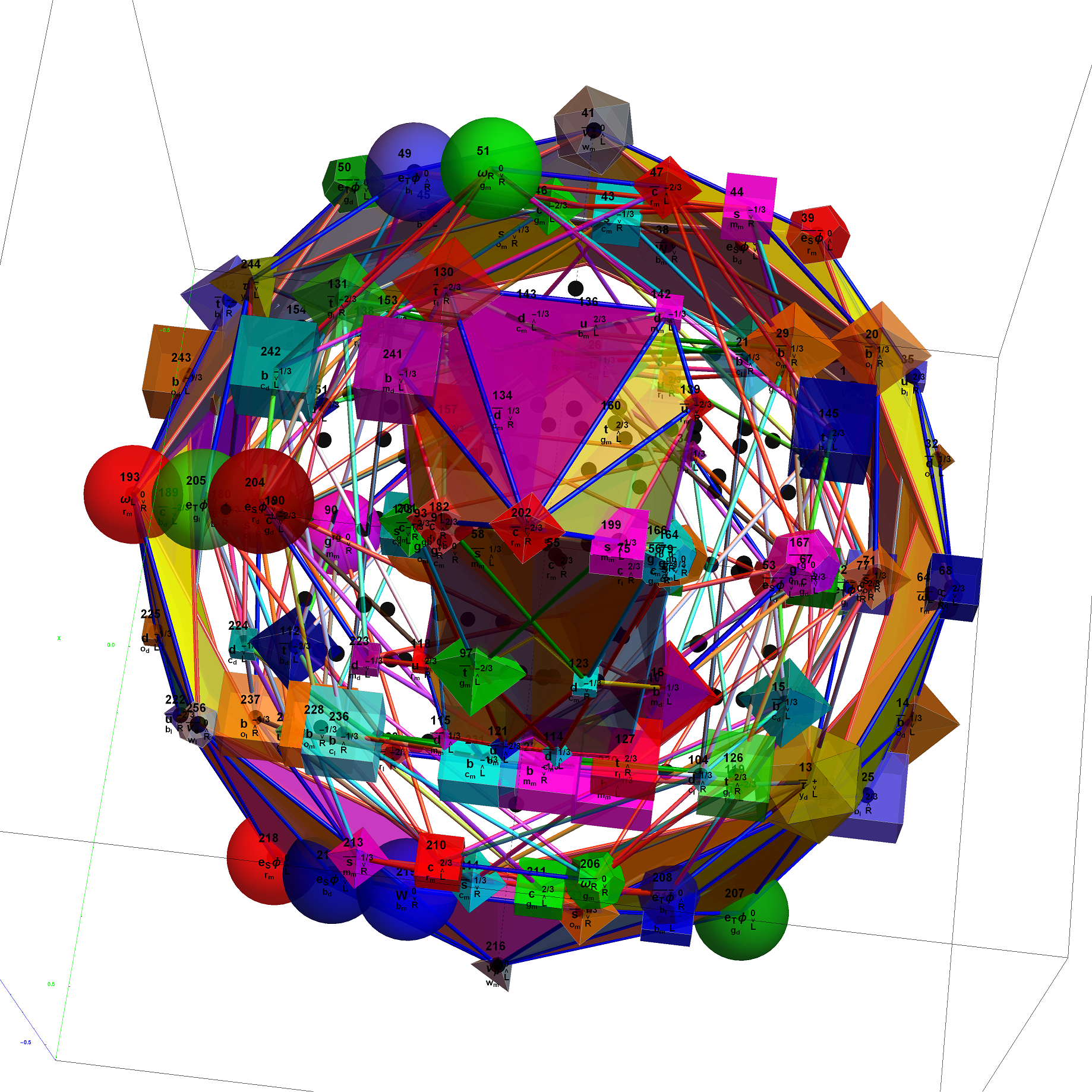
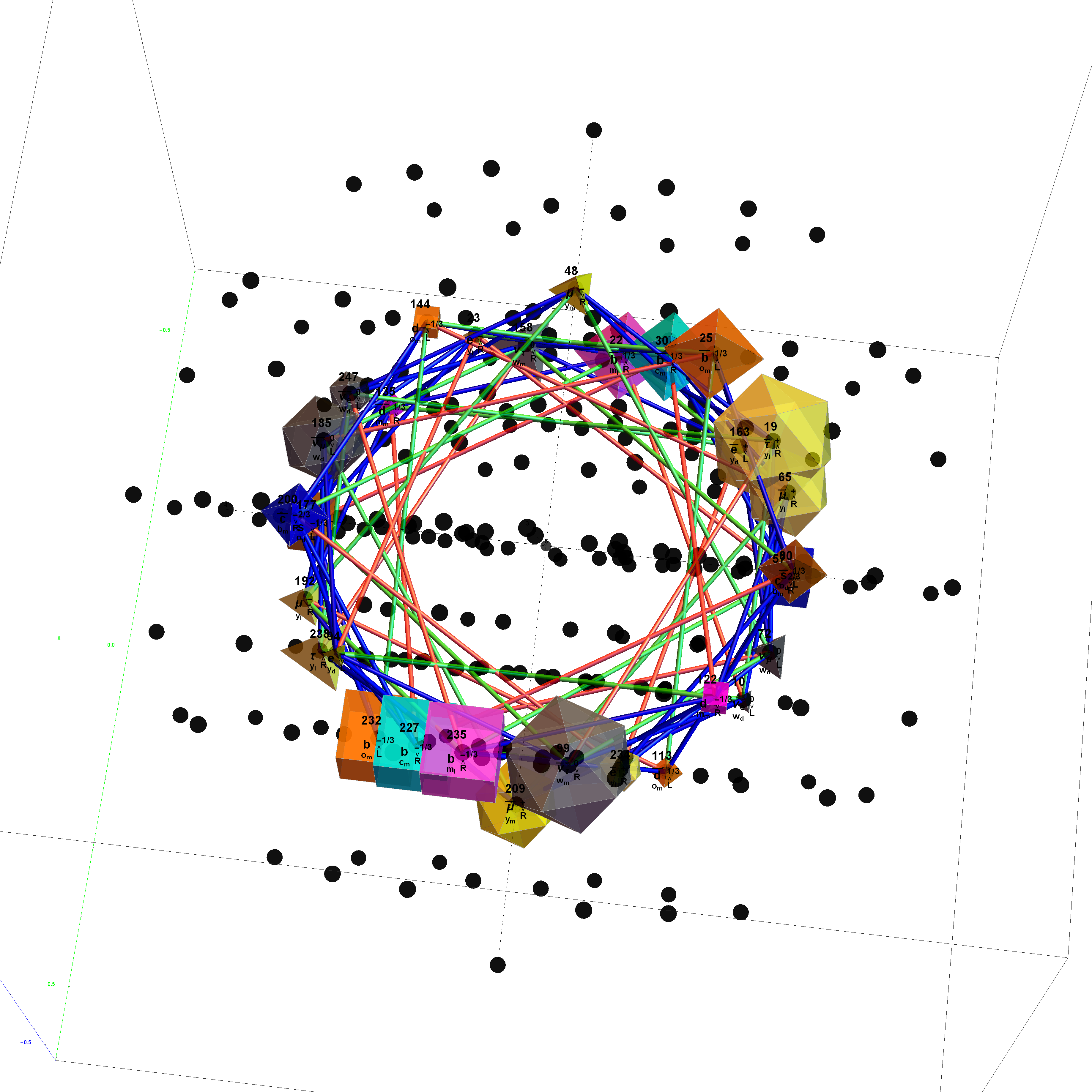
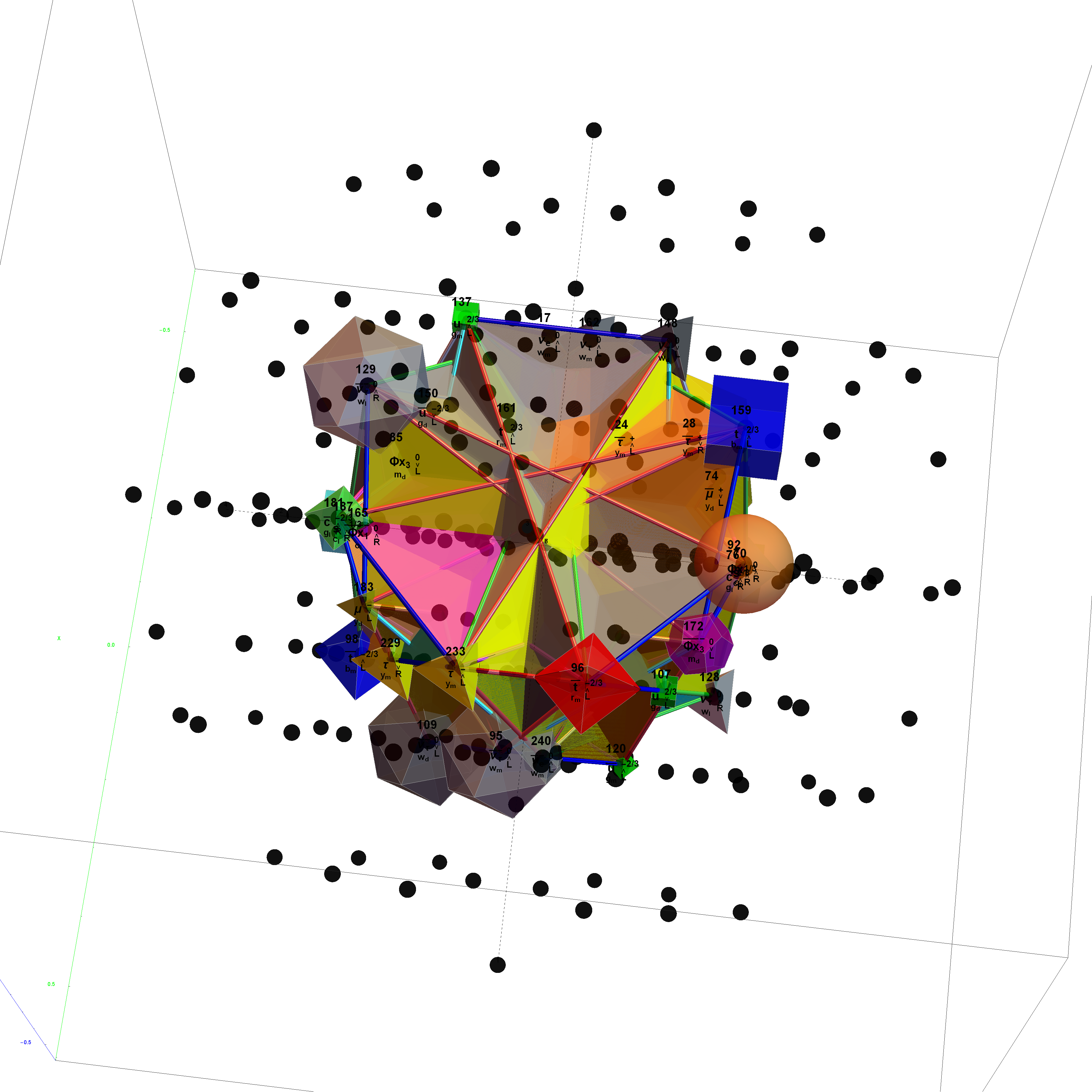
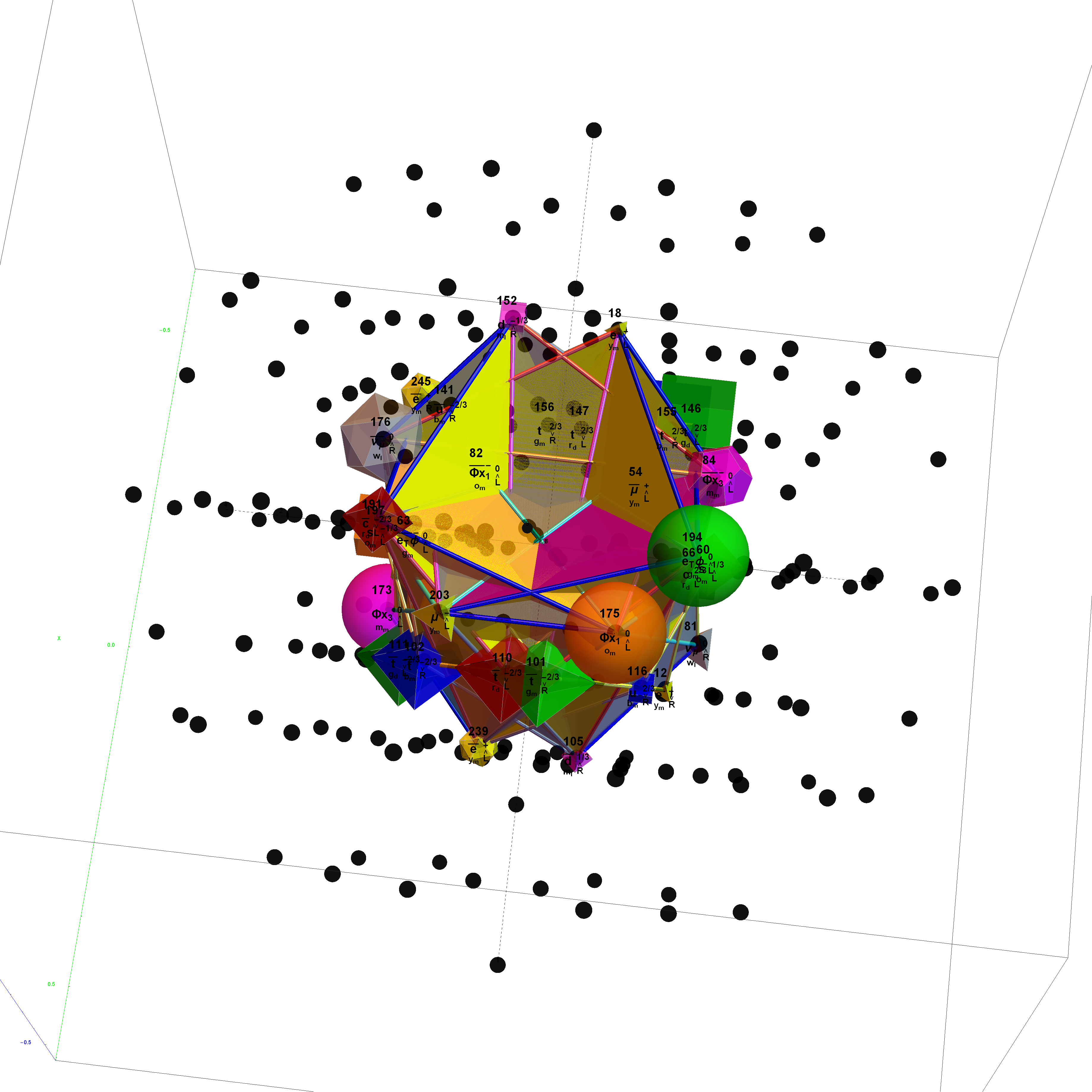
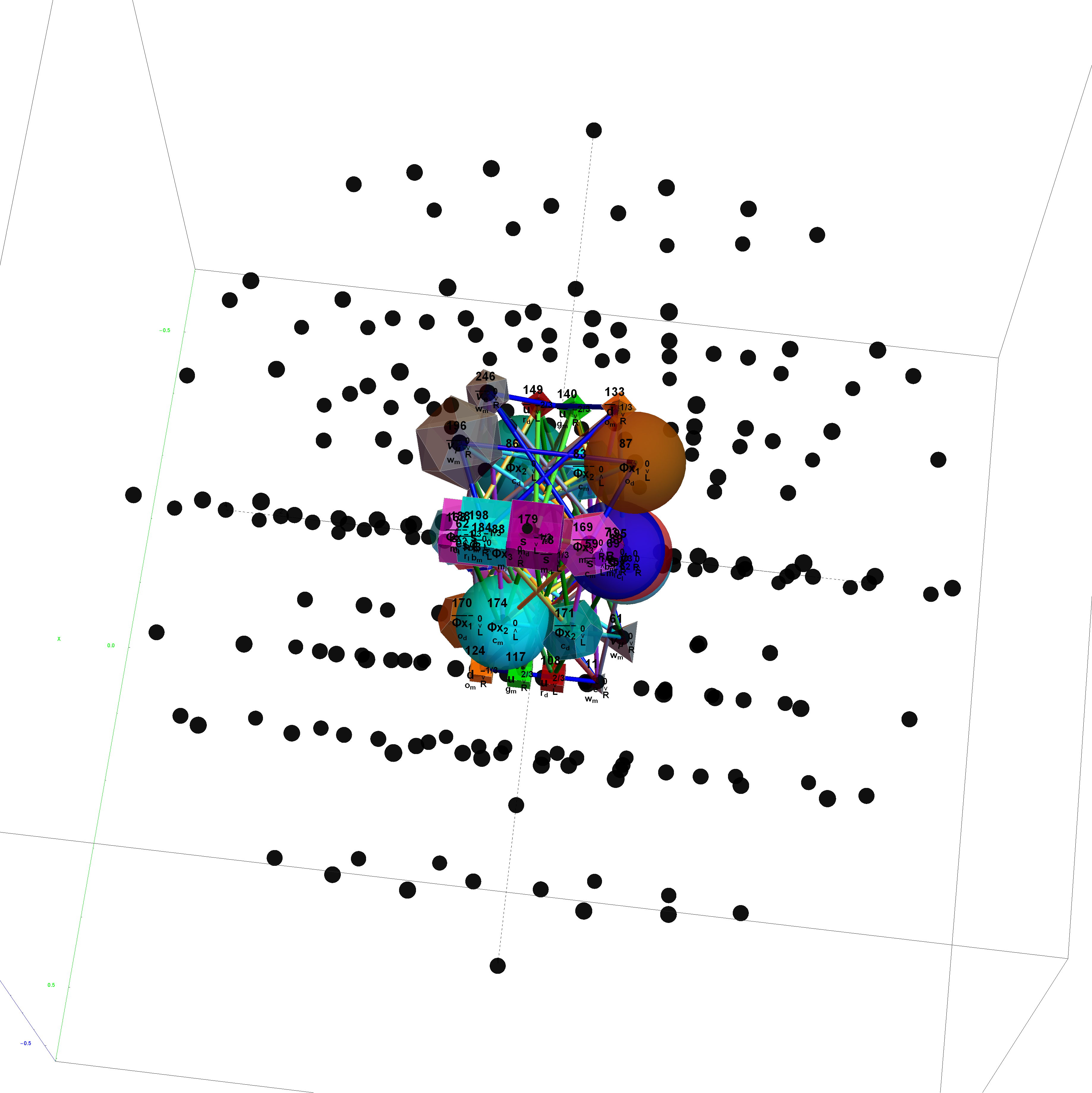
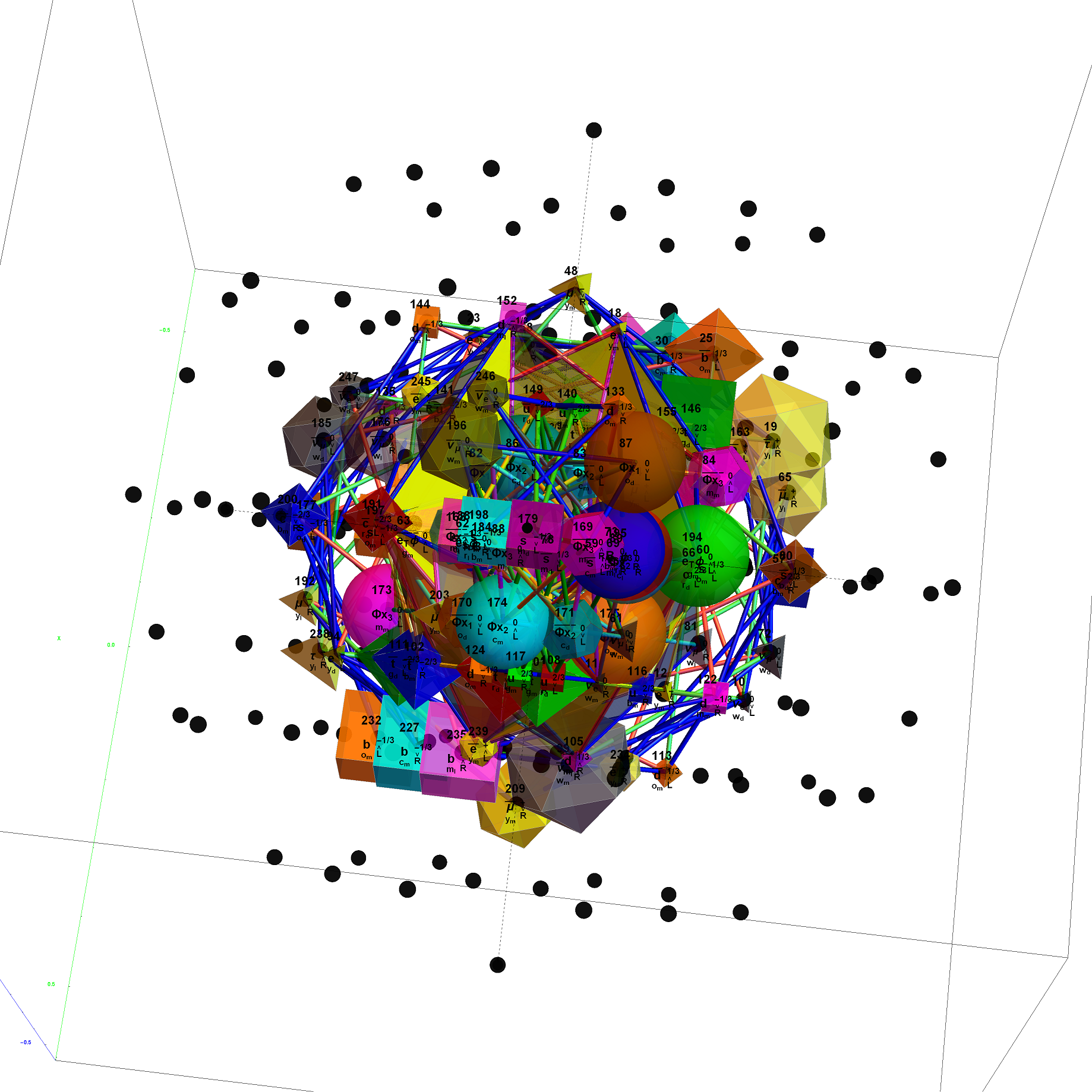
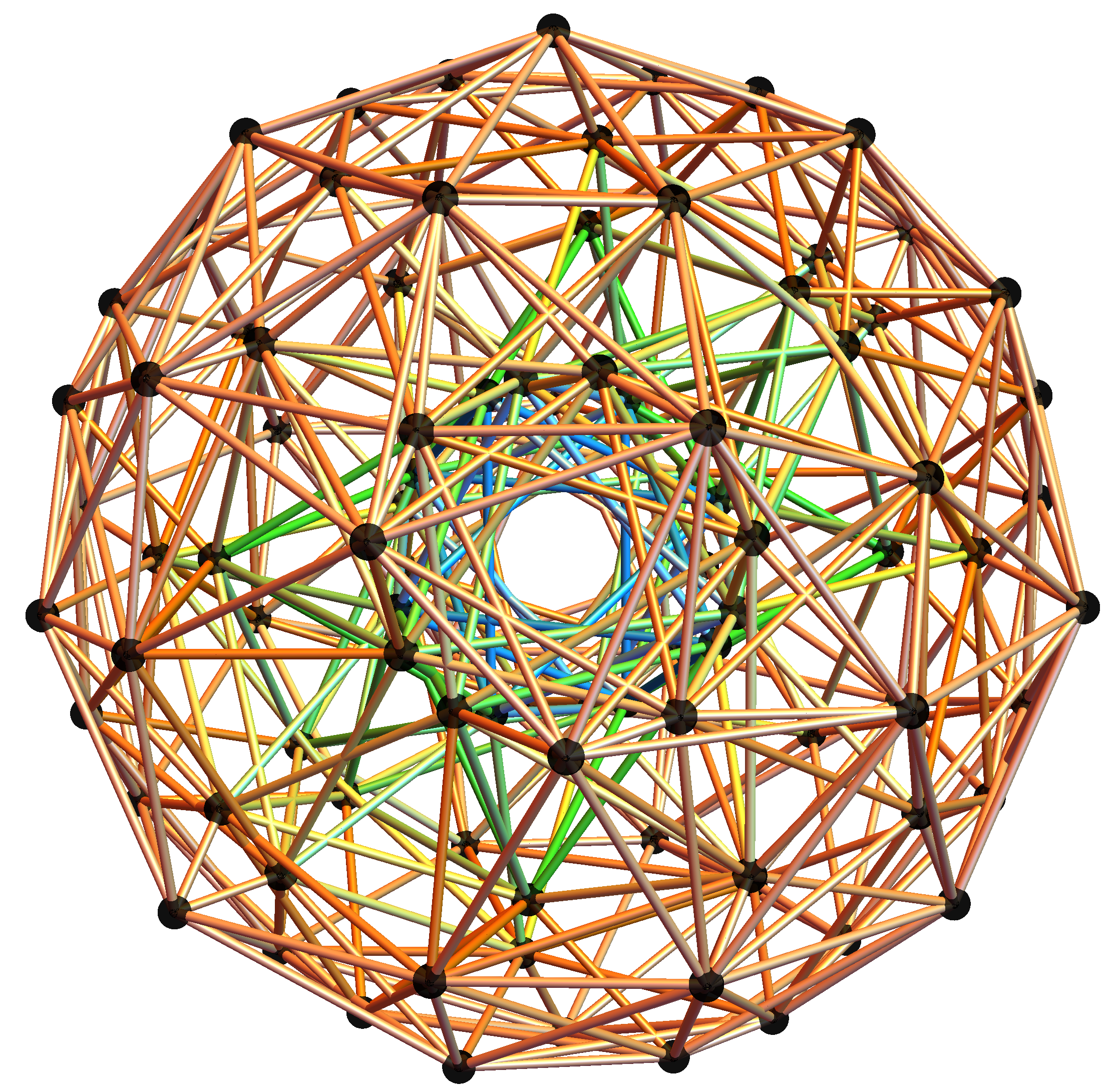
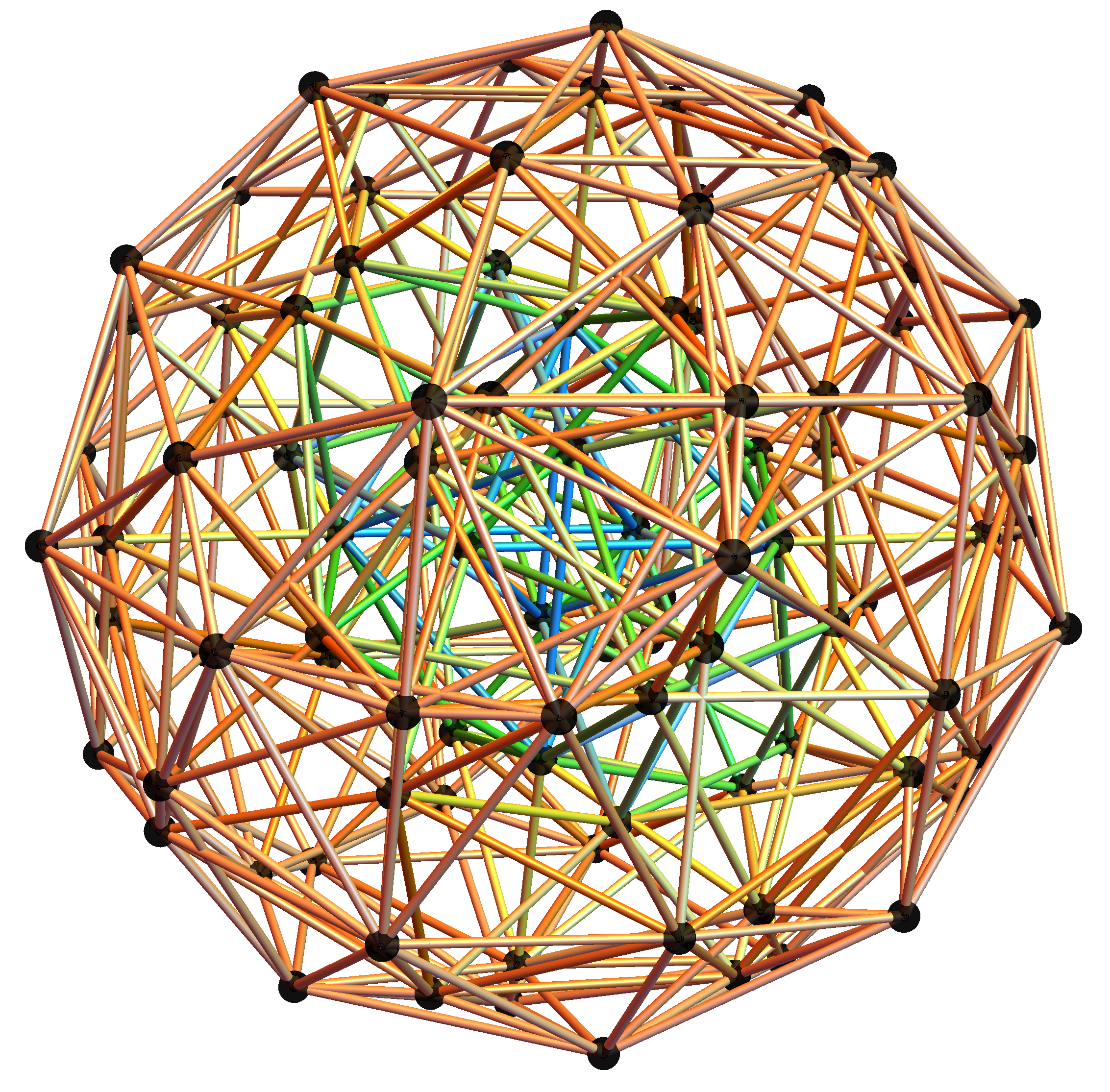
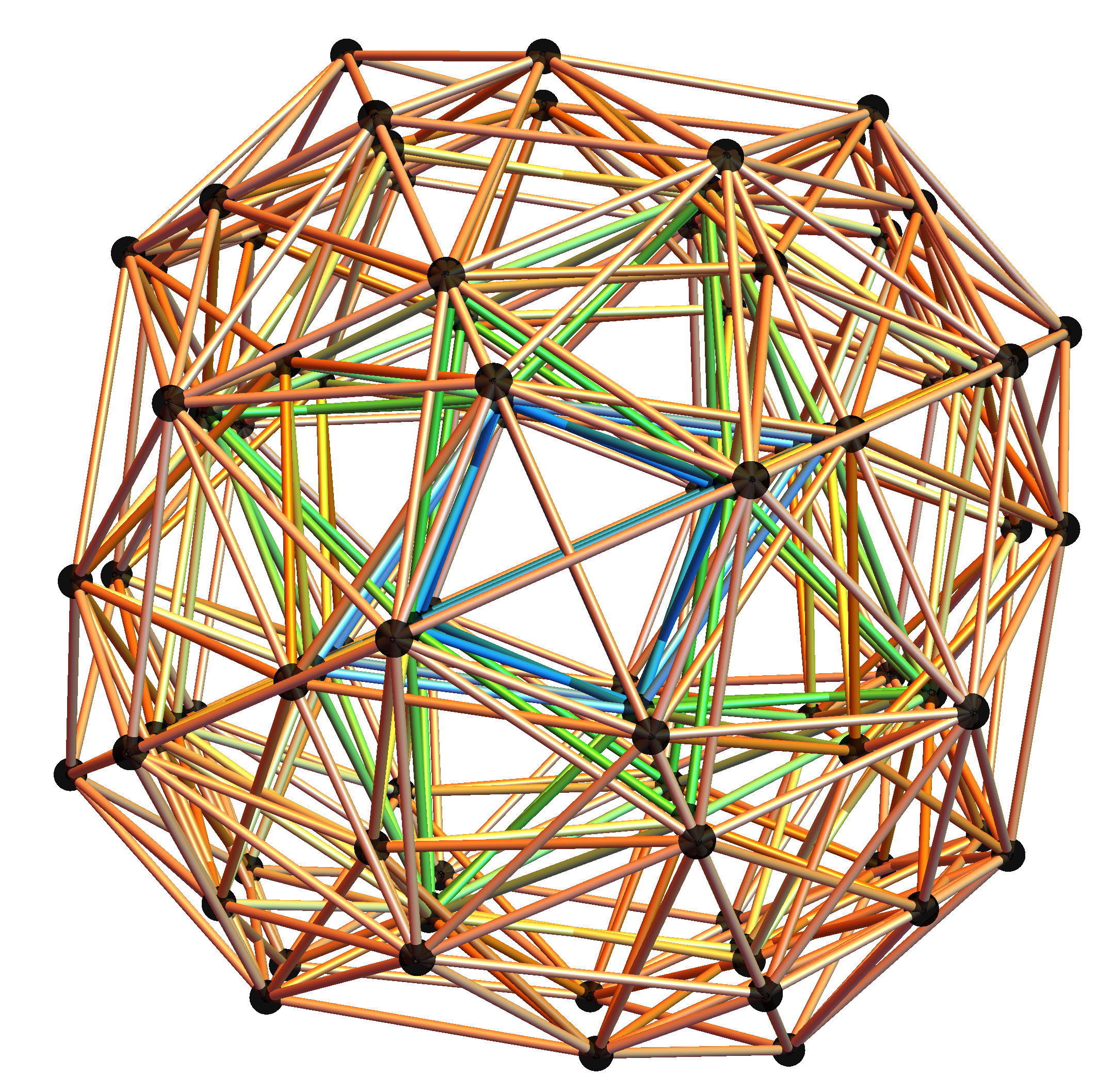
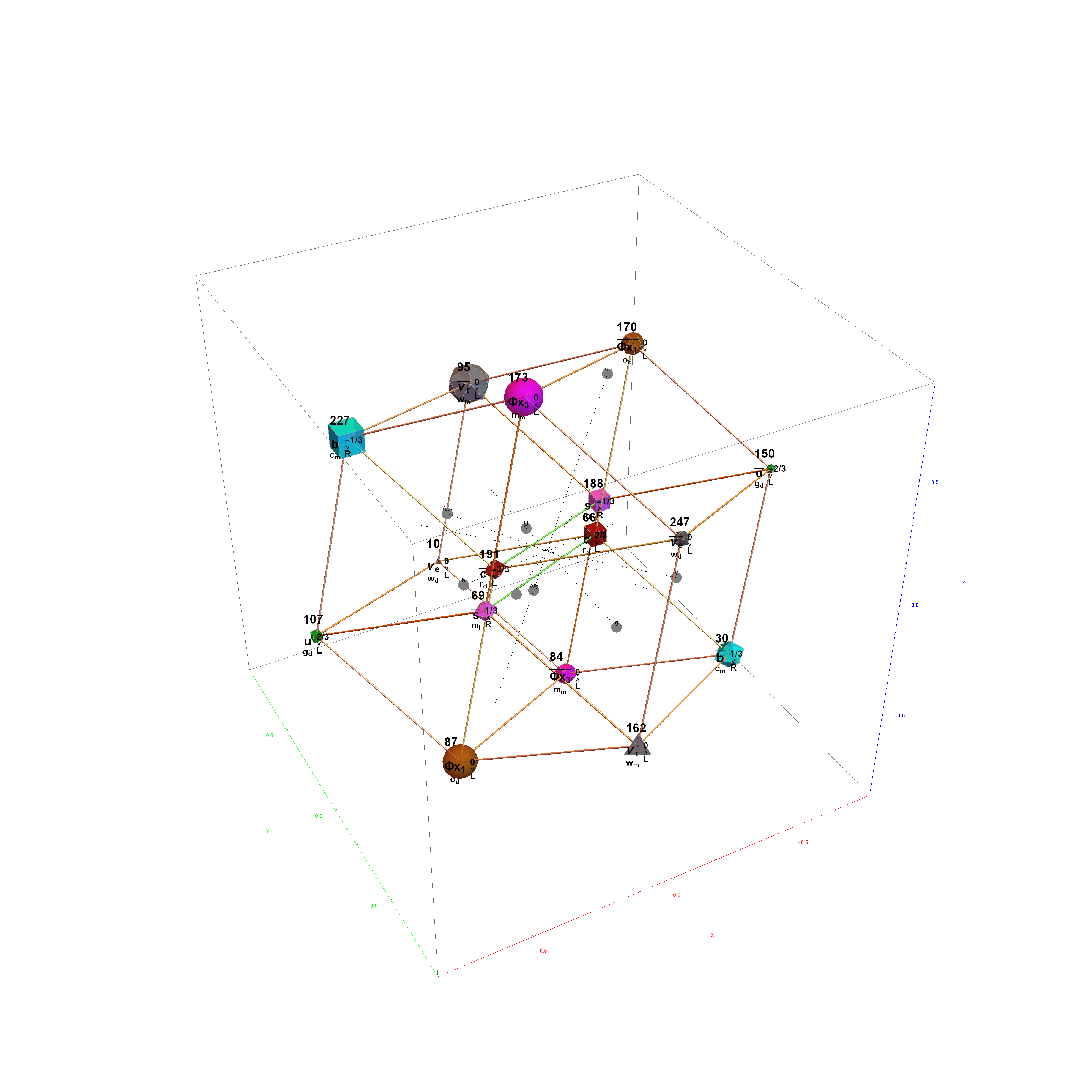
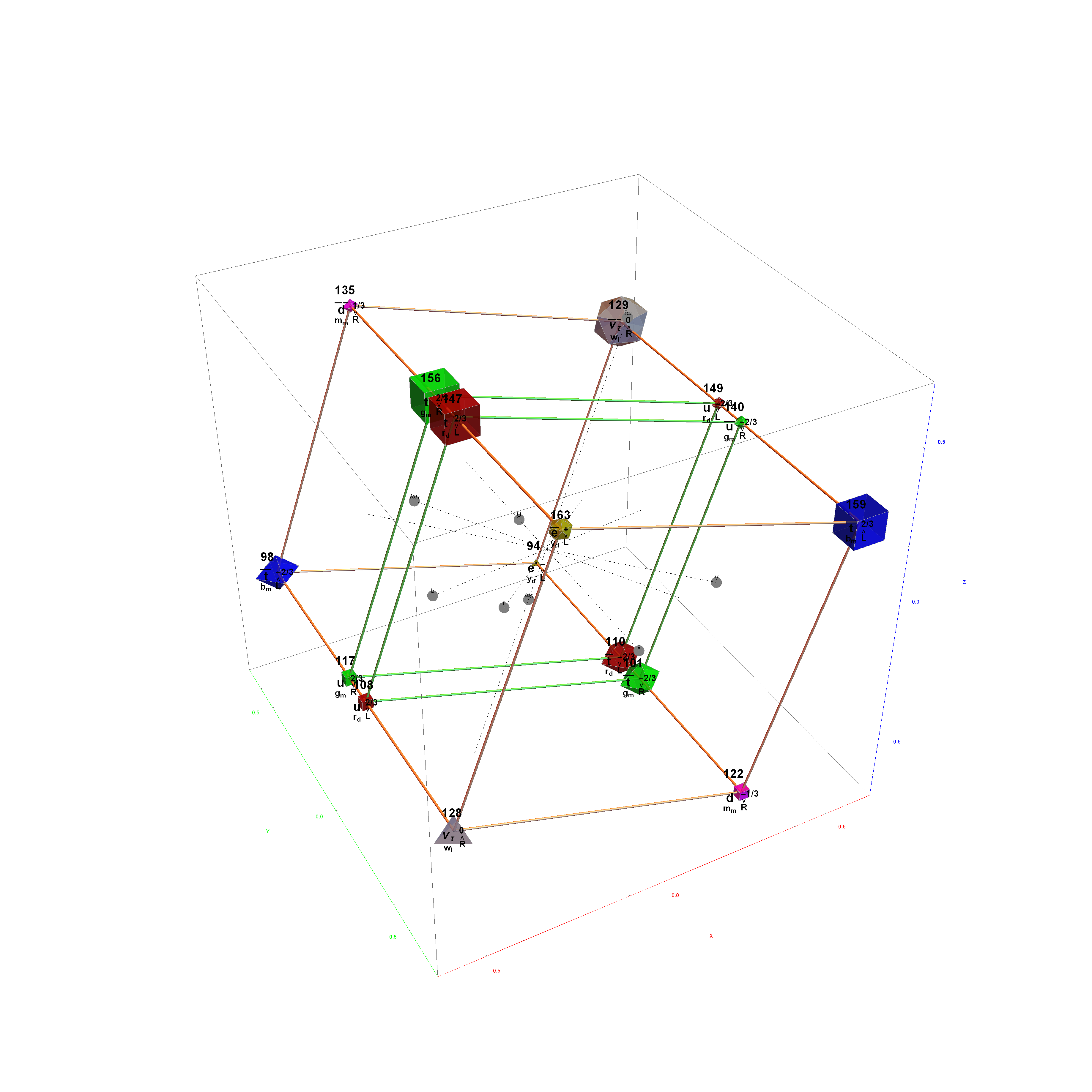
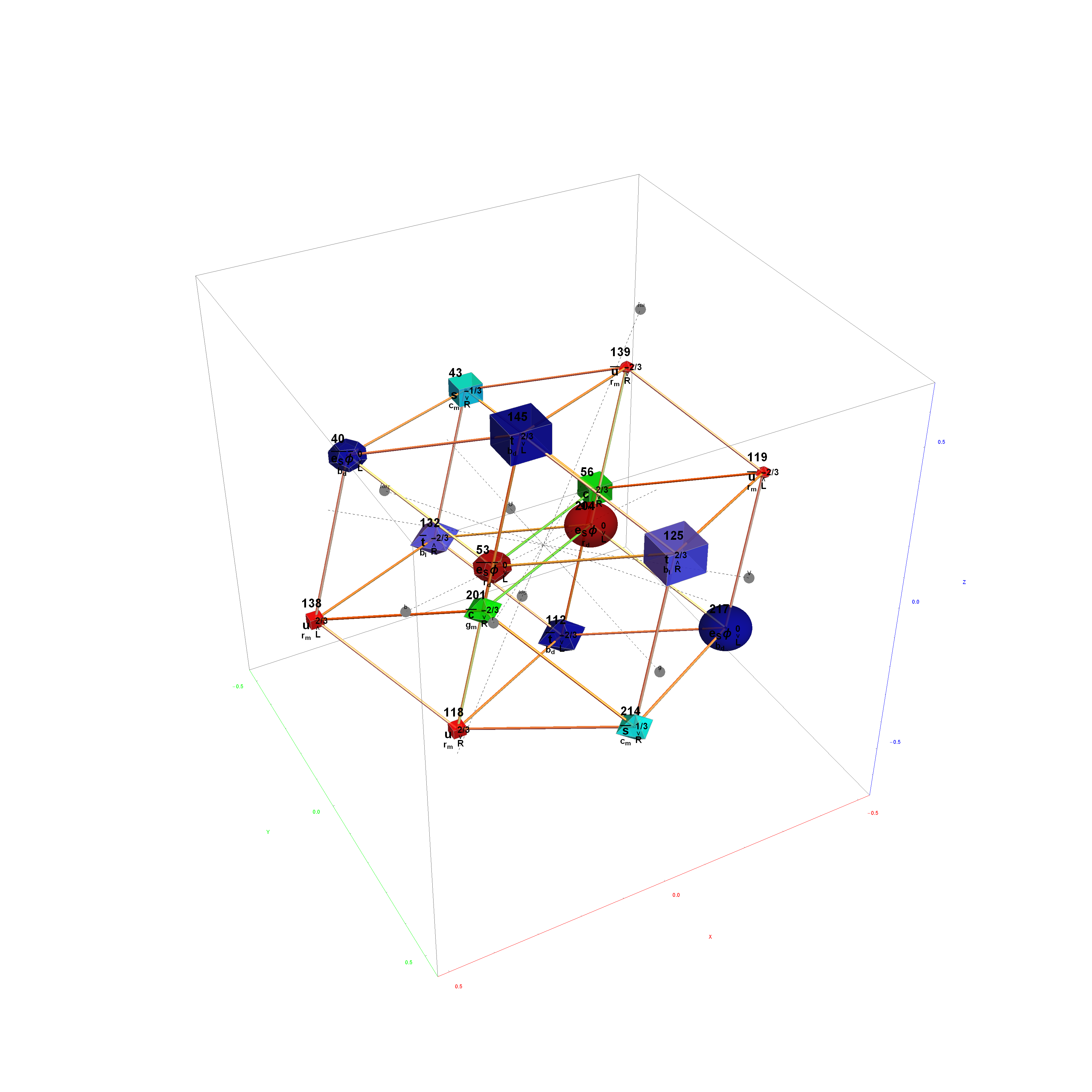
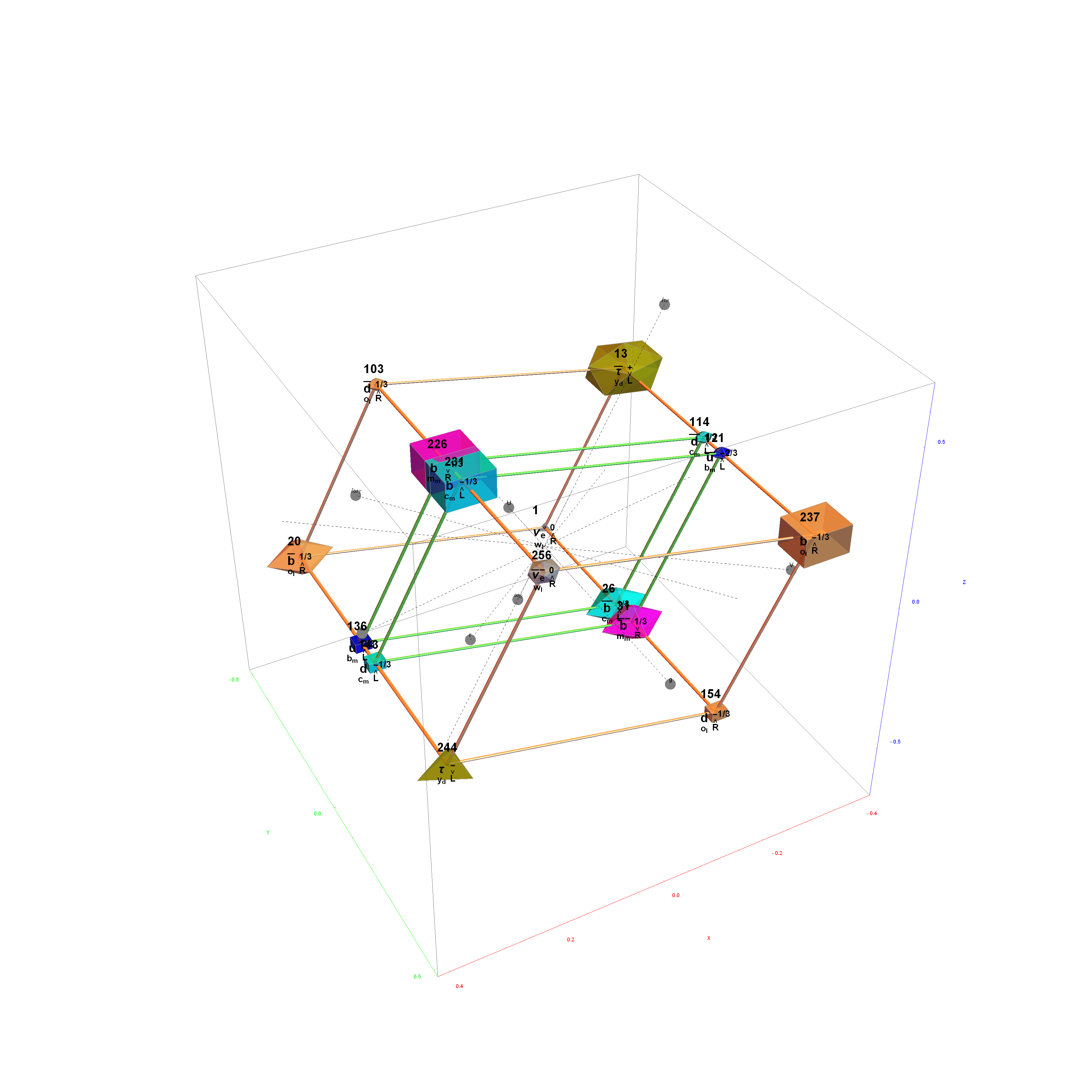
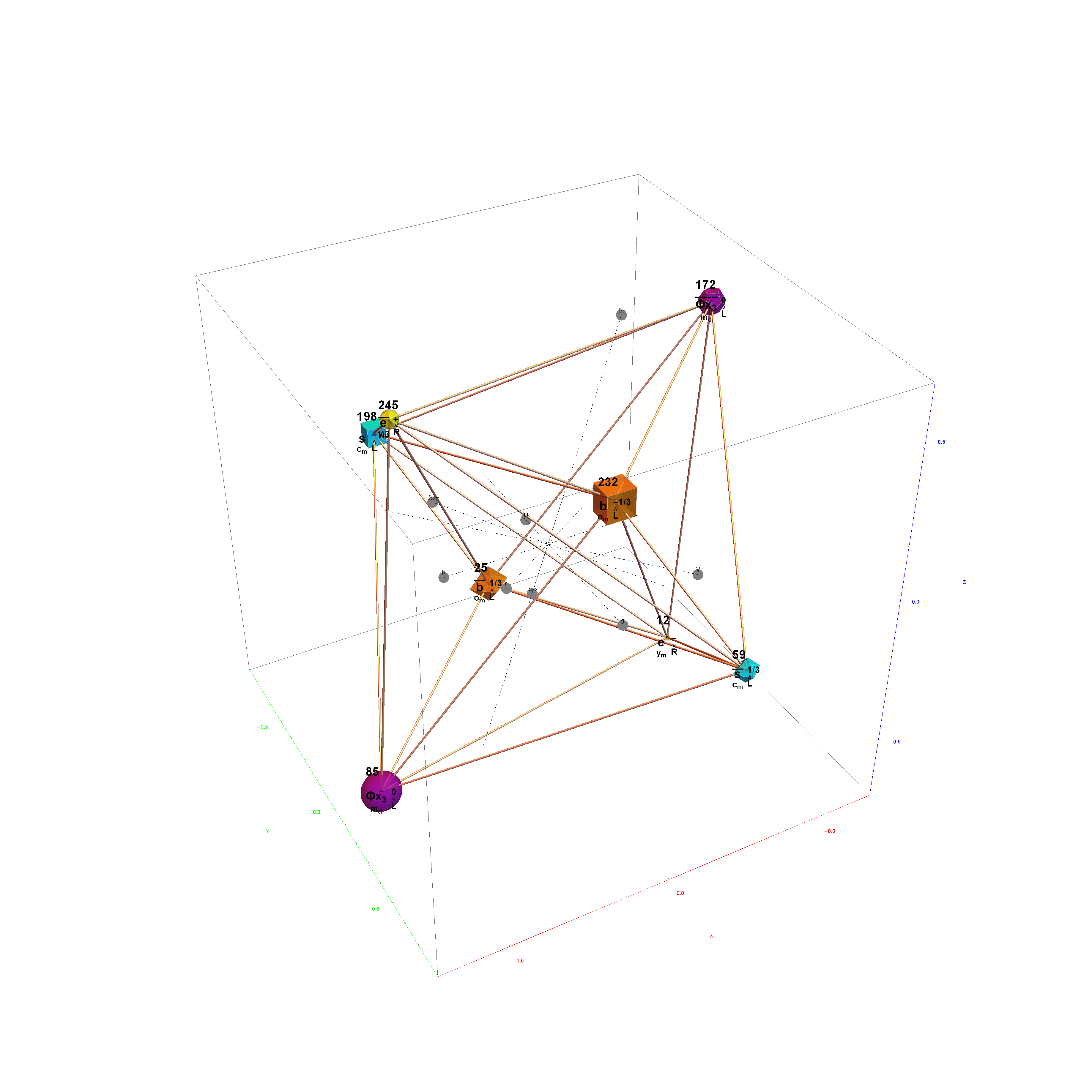
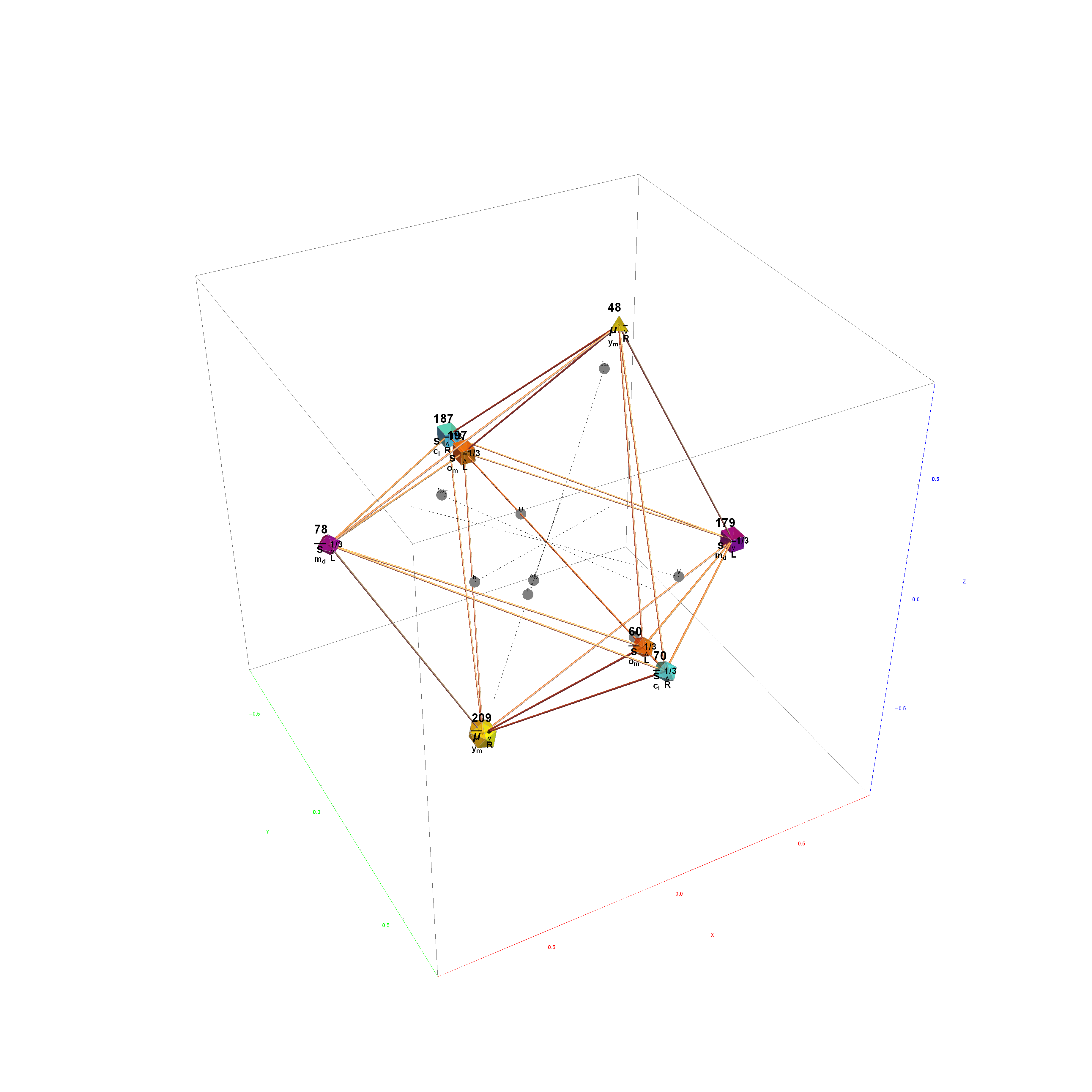
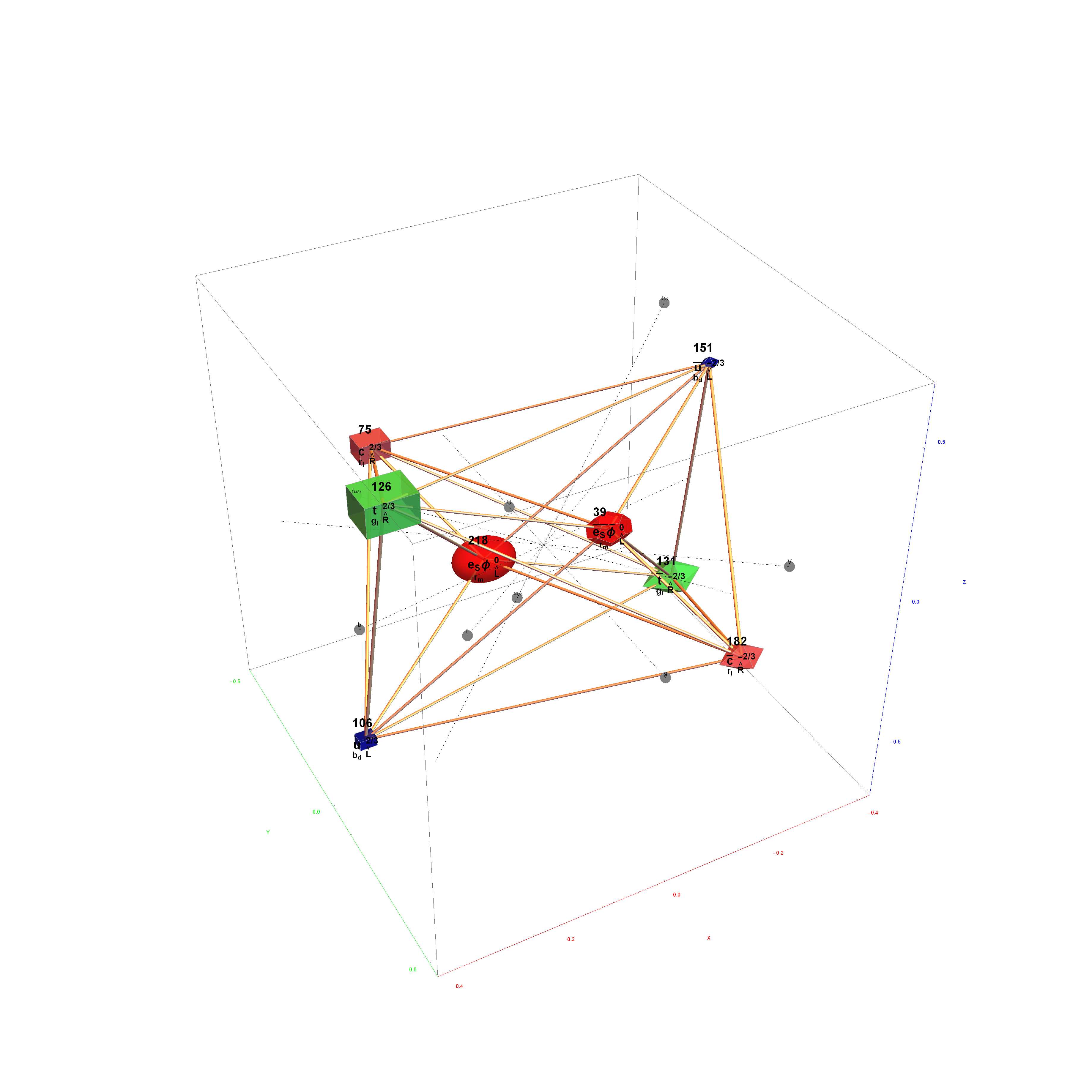
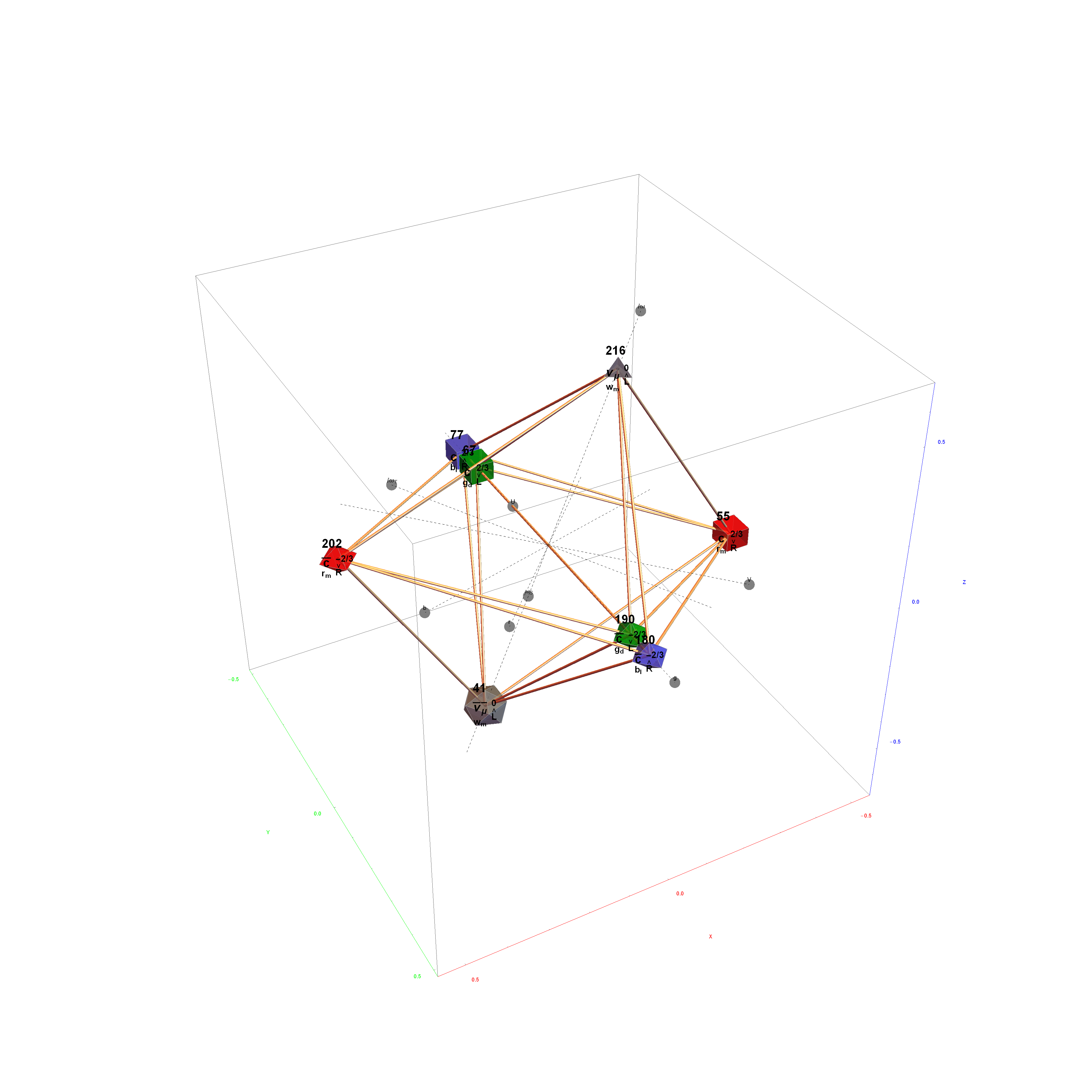
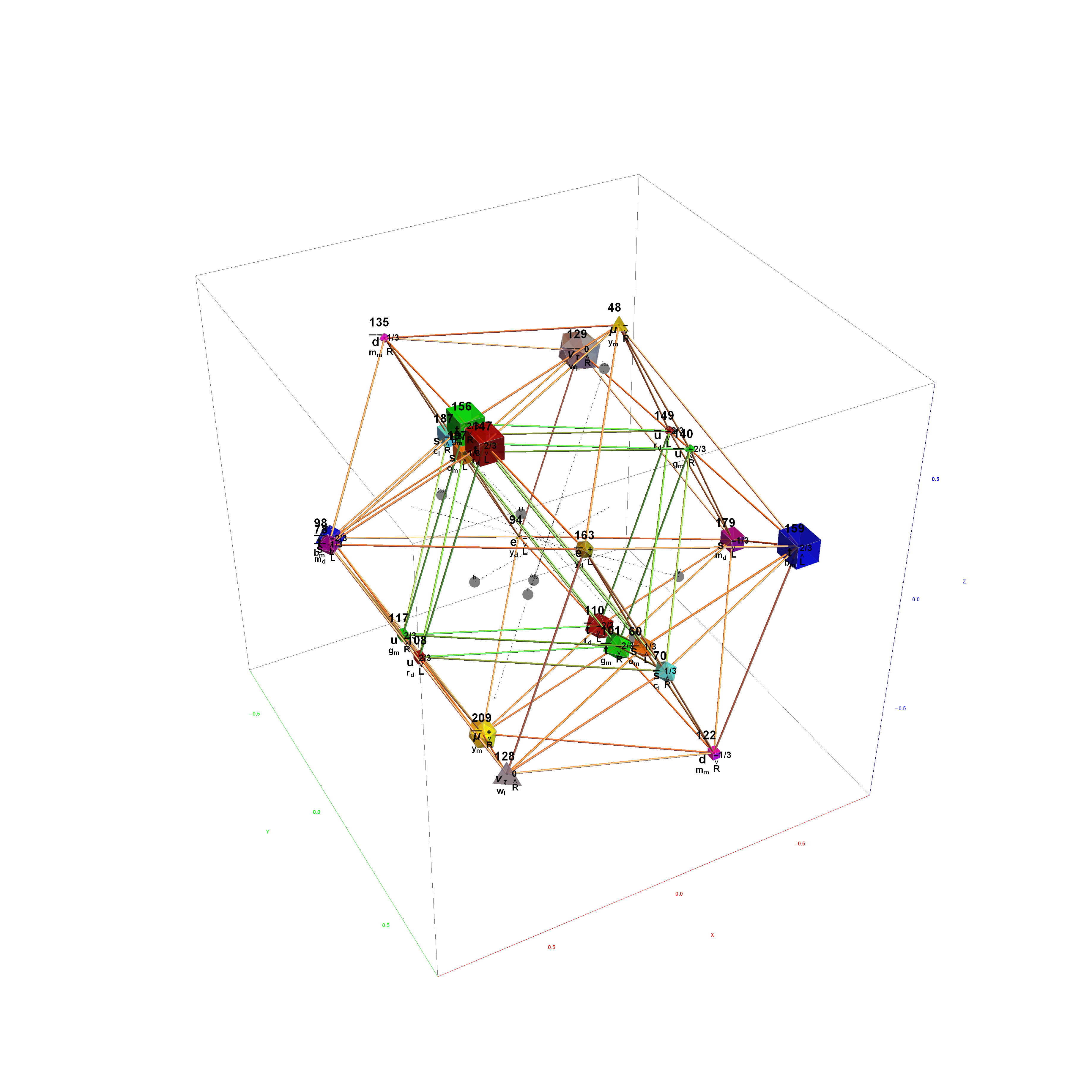
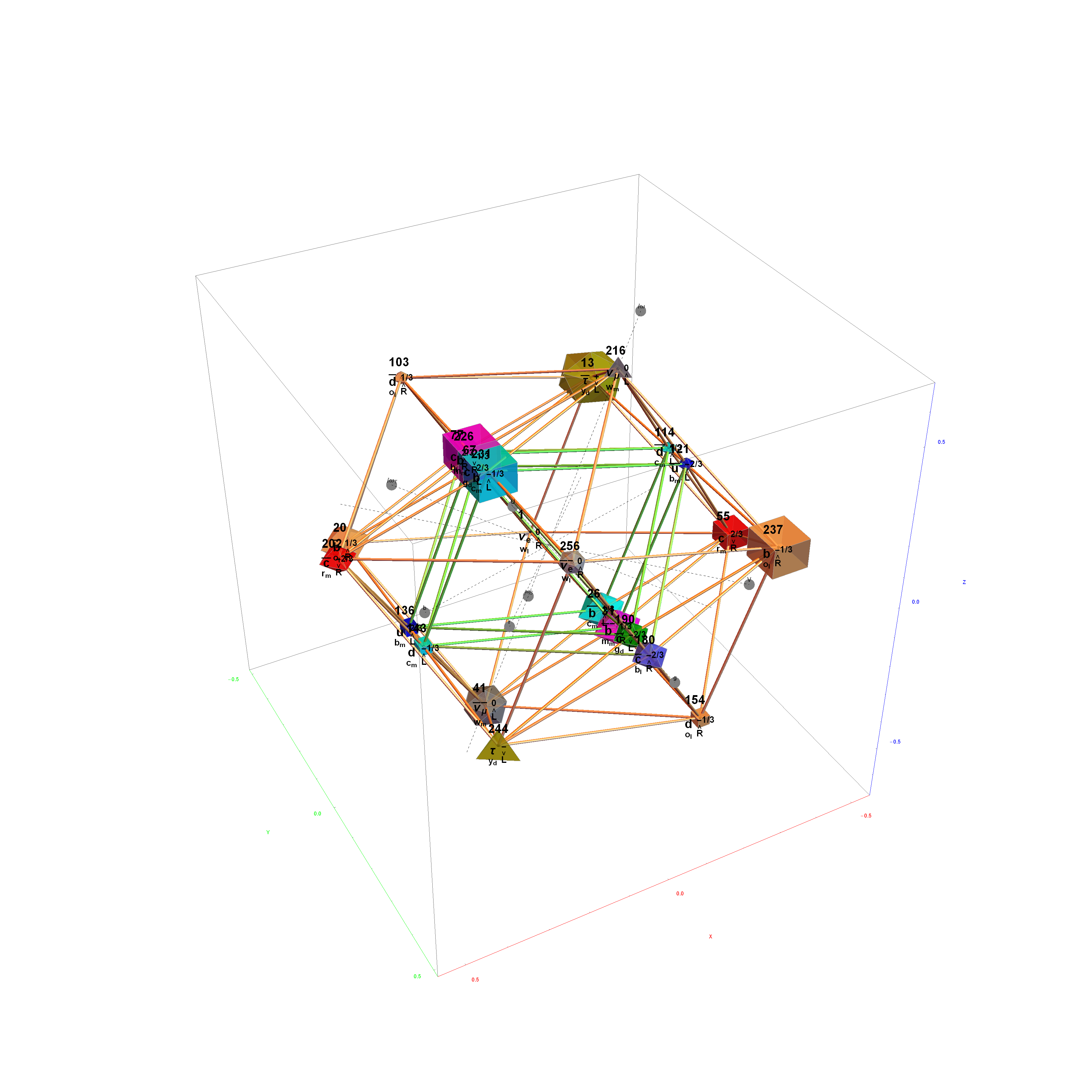
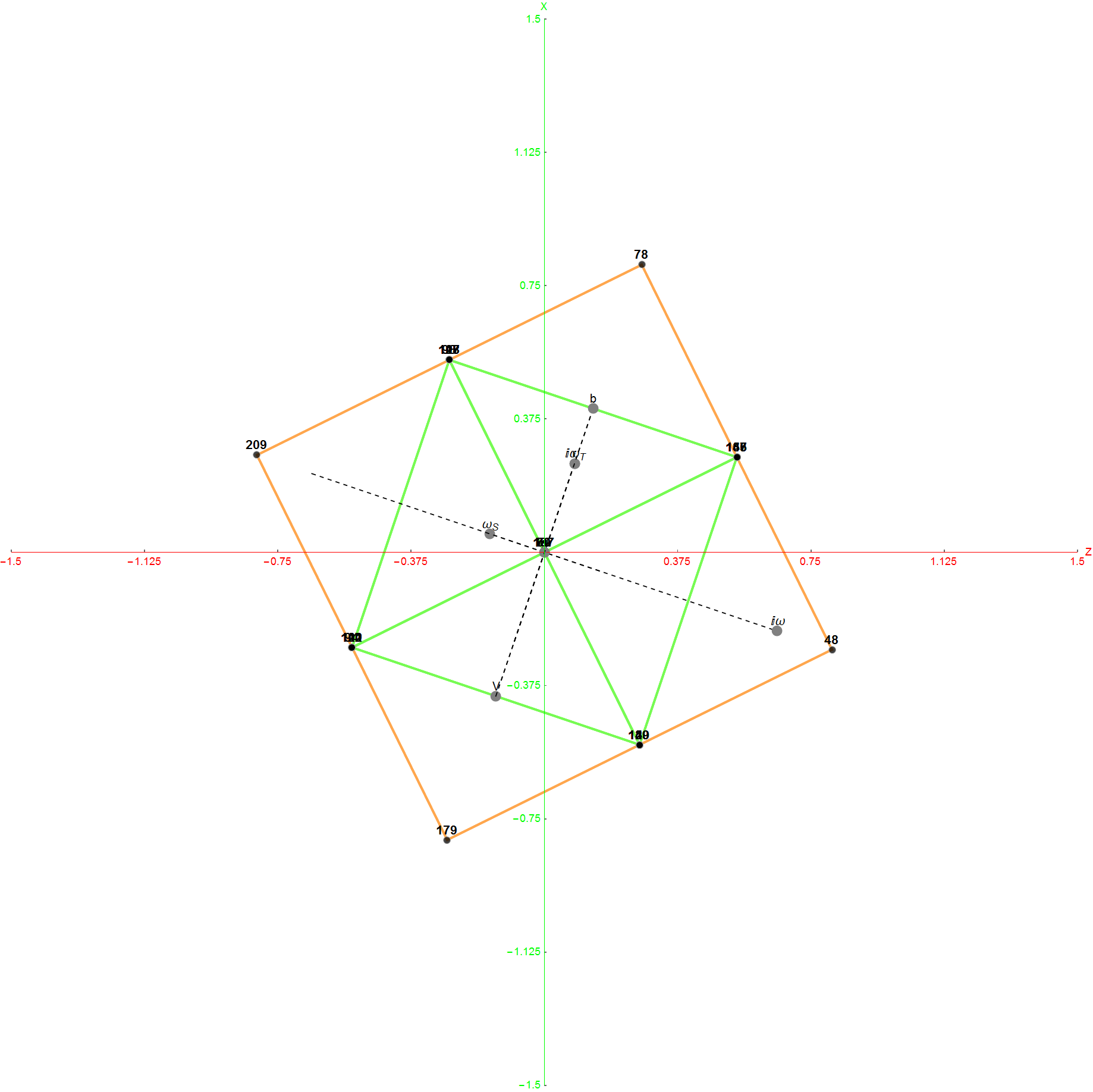
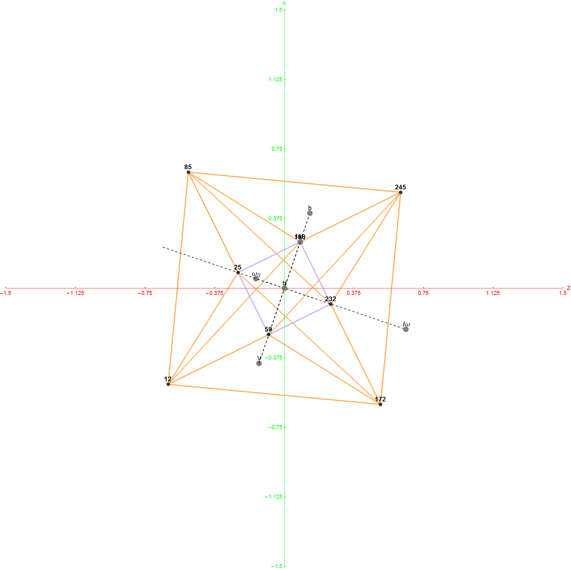
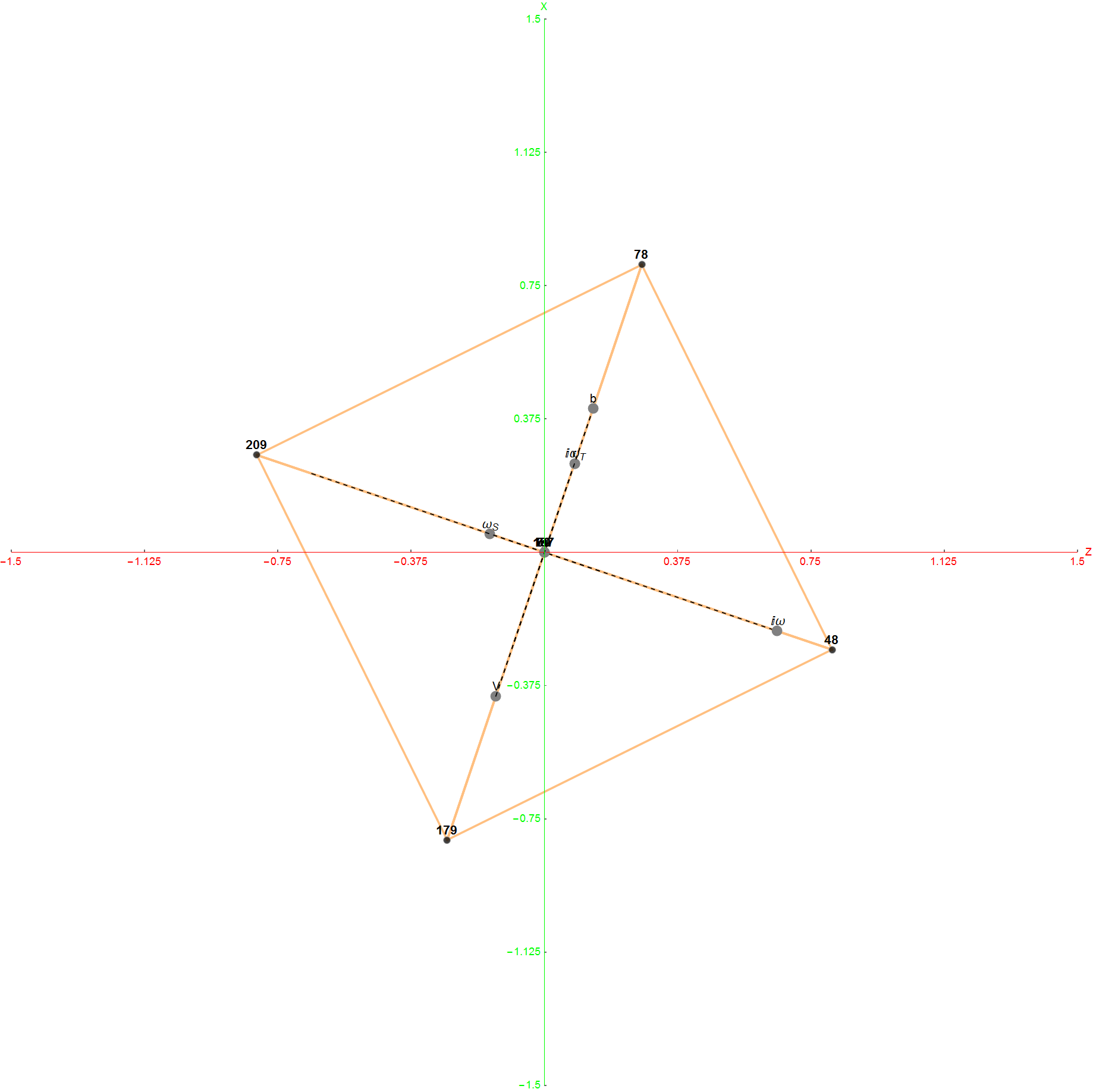
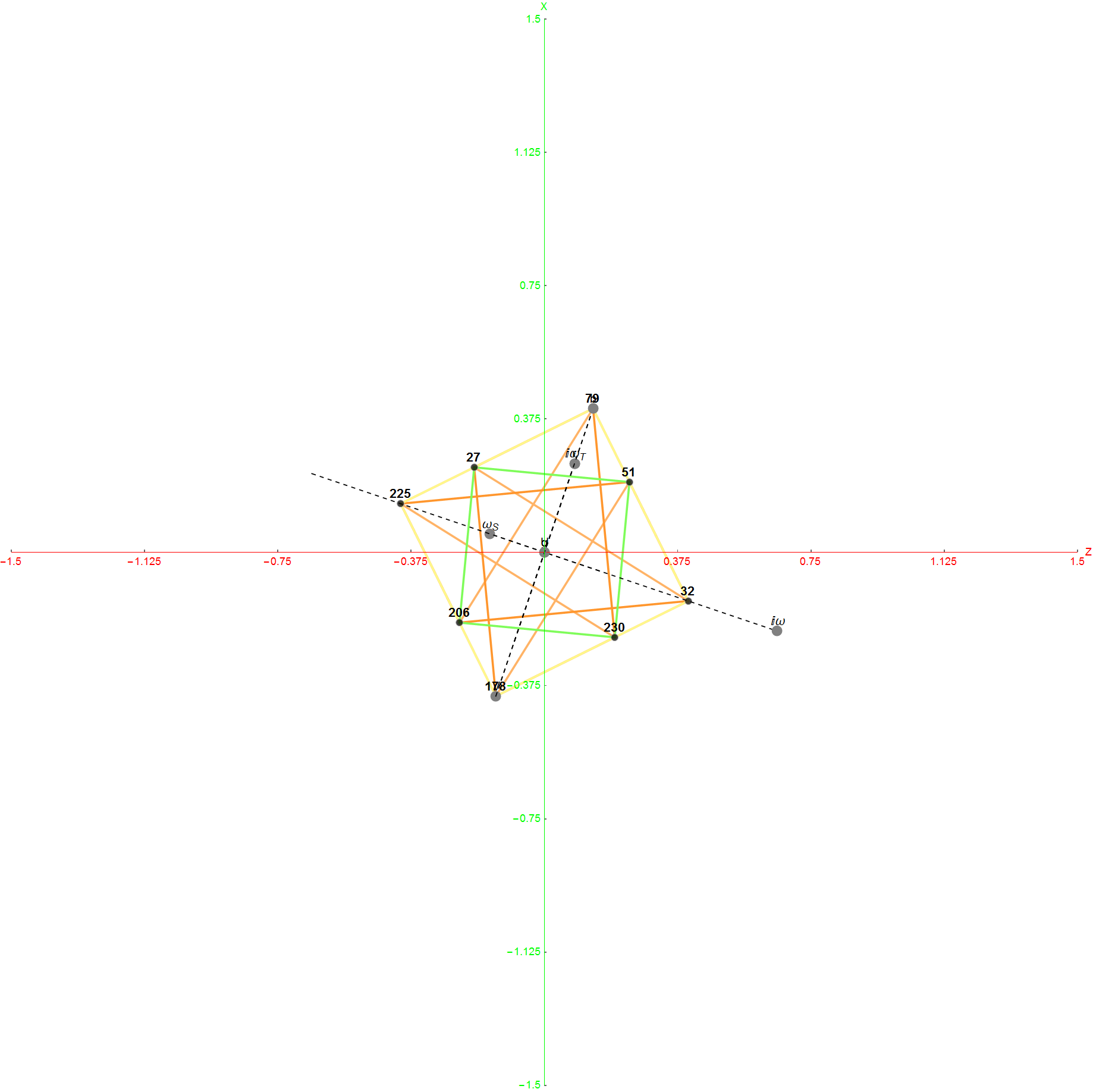
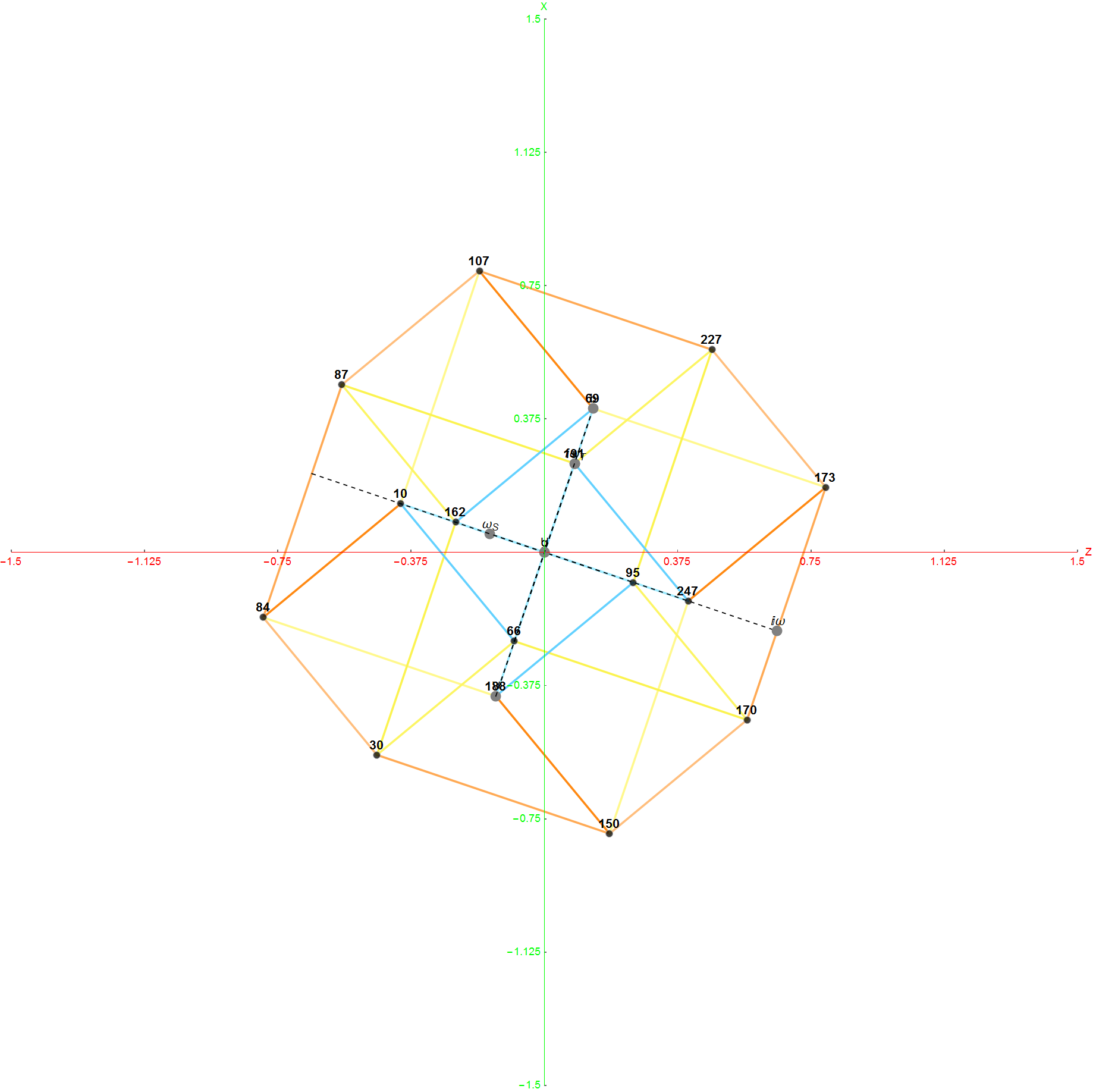
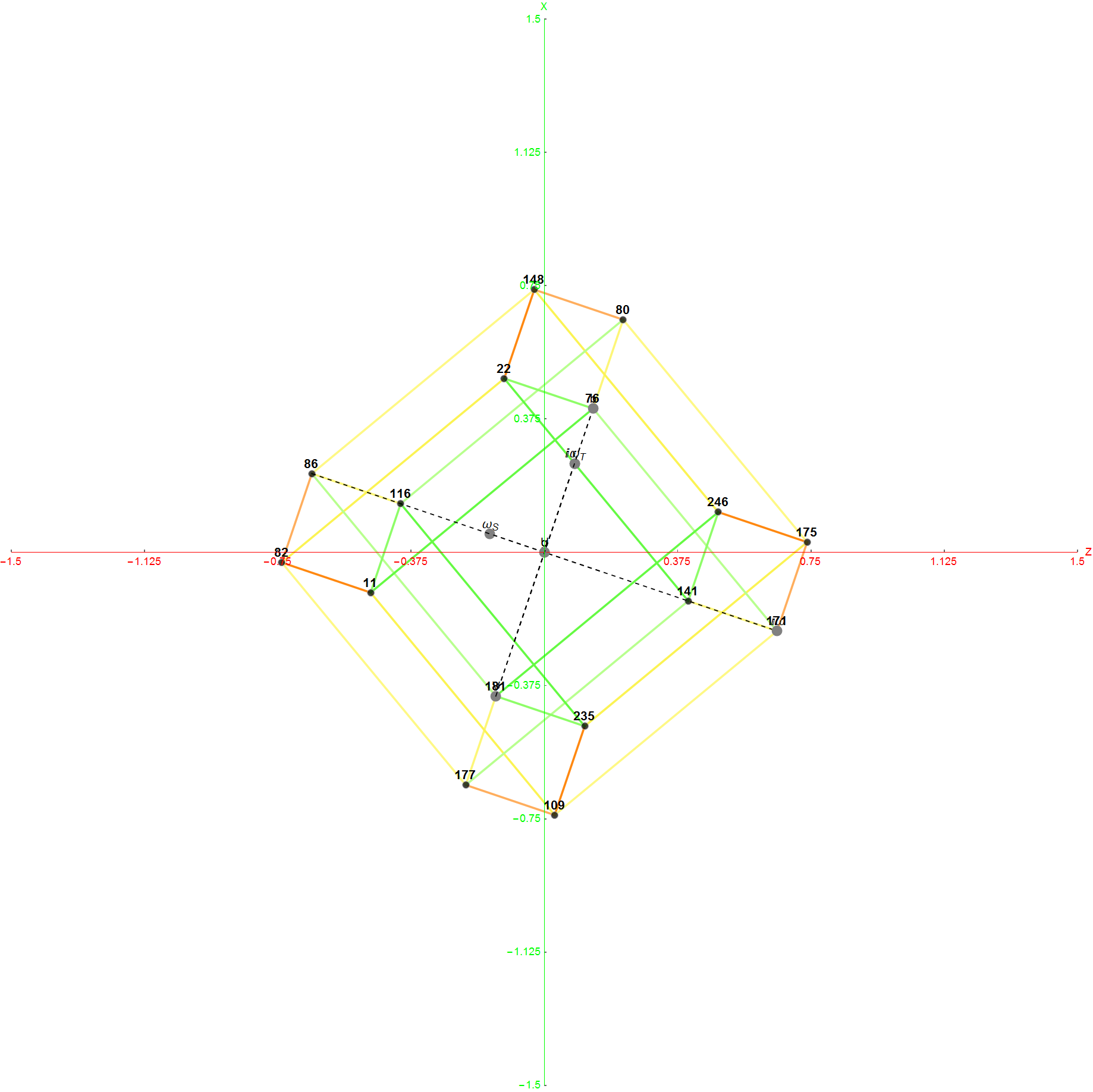
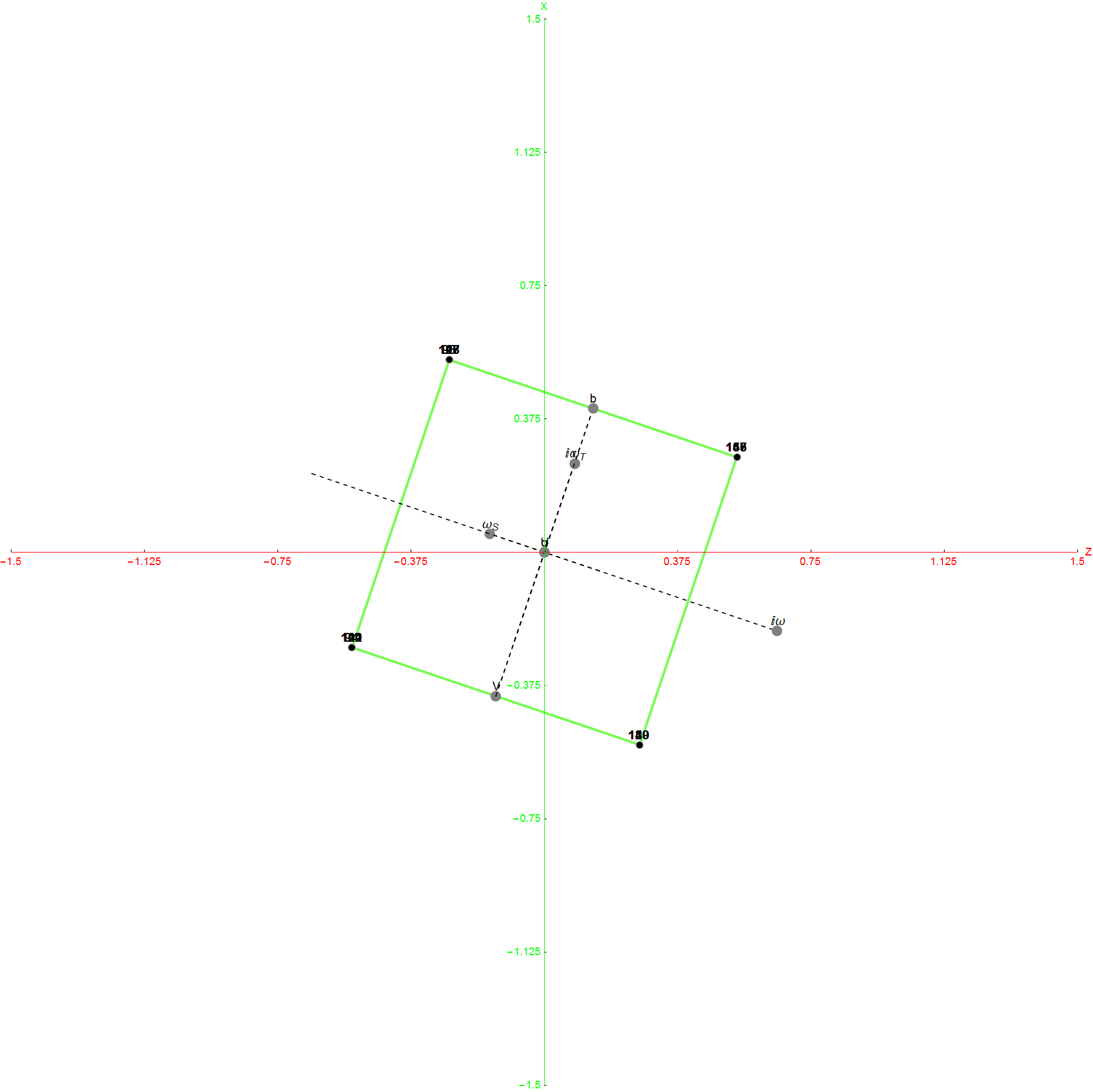
Viewing the static or animated 2D (or 3D) positions of selected vertices (or their theoretically assigned fundamental physics particle) is accomplished by projecting them using a dot product of 2 (or 3) 8D basis vectors. These can be manipulated with controls in the HMI pane 8. 3D displays use native Mathematica rotation and zoom options (cntrl or alt-click-drag)
The triality buttons “T1”, “T1p”, “T2”, “T2p”, “T4”, and “T4p” select different sets of triality rotations using one or more of the selected rotation matrices. These are named for the number of sixths of a unit circle involved in selected hyperplanes of a higher-dimensional rotation. The suffix of “p” indicates that it uses the “physics” data set, which is a rotation of the SRE E8 vertices that let A. G. Lisi calculate particle charges on a single generation of fermion particles. The physics data set is activated in some “Favorite” selections.
Animations are generated by increasing the number of (time) steps and selecting the type of 8D “flight path” (Translational or Rotational and Spin – controlled in the HMI pane 8).
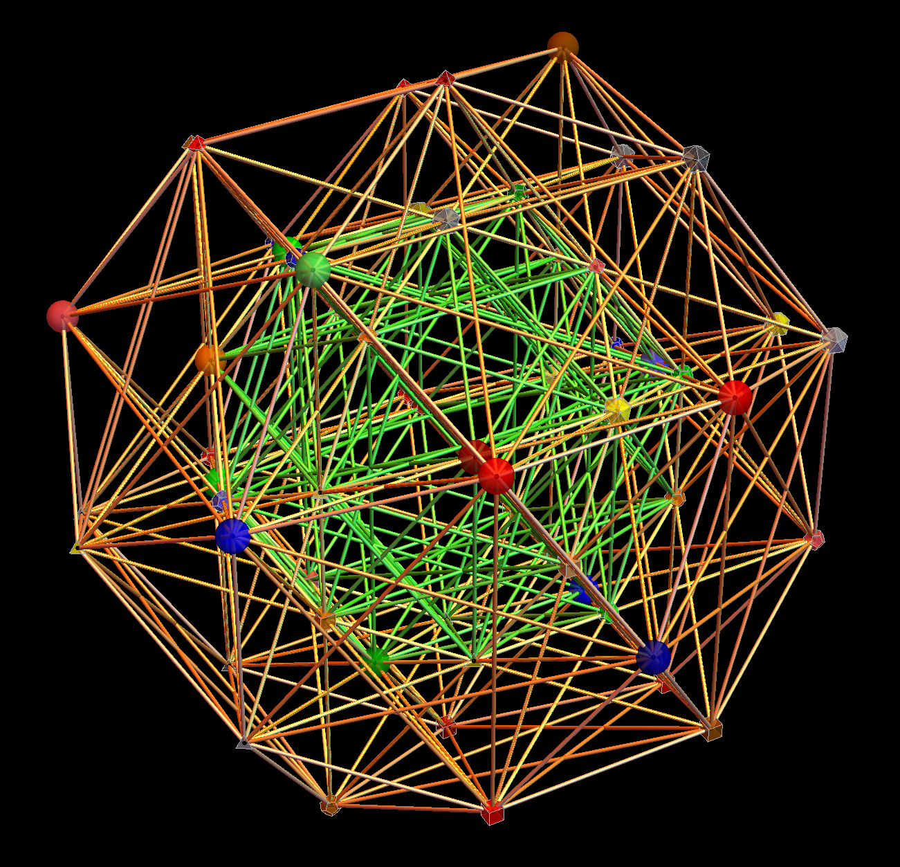
It is interesting to note that the 8D vertex positions are always static. What is moving is the 2D (or 3D) perspective inside an 8D “information space”. The “information space” in this case is made up of the highly symmetric vertex positions of the Split Real Even (SRE) E8 Lie Group assigned to fundamental physics particles based on their quantum numbers. The specifics of each flight path are depend ant on the 3 basis vectors and dimensions selected for creating the hyper – planes about which they rotate. These are also manipulated with controls in the HMI pane 8.
Mouse over the shapes in the result to show the detail particle information relating to E8, Cellular Automata and physics (as shown in the “Particle” pane 4).
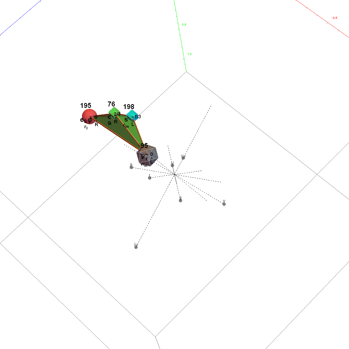
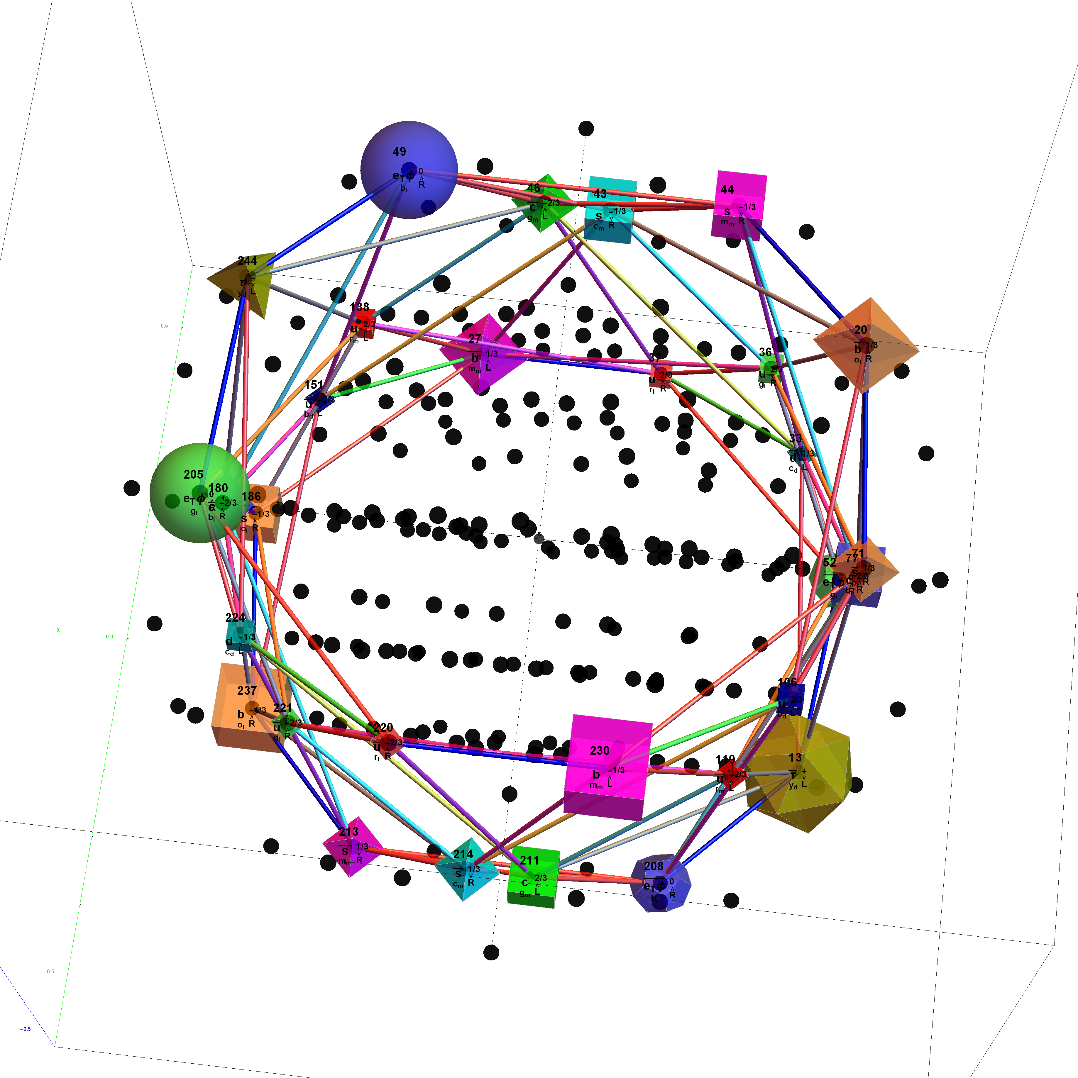
The output window is a clickable pane (if in 2D mode). If the physics box is not checked (showing vertex dots), clicking on or near a vertex calculates and shows the connecting vertex edges of the (nearest) clicked vertex. The edges are color coded by overlap count. If the physics box is checked (showing assigned particle shapes), clicking calculates triads of edges that include the particles whose E8 vertex values sum to the clicked particle. Clicking an already highlighted vertex now shows only that edge (or triad of edges).
Edge calculation is done with a modified code snippet from Eric W. Weisstein, “600-Cell.” From MathWorld – A Wolfram Web Resource. http://mathworld.wolfram.com/600-Cell.html
If you have Mathematica and want to get a more fully interactive experience, simply set “localize=False” near the top of the initialization section. This activates many features not available in Demonstrations.
References
[1] A. G. Lisi. “An Exceptionally Simple Theory of Everything.” (Nov 6, 2007) arxiv.org/abs/0711.0770.
Particle:
This demonstration creates an interactive pane for identifying fundamental particles in physics through the selection of quantum parameters. The information displayed in the output window is also displayed in the ToolTip on mouse-over of the particles in the E8 window.
It includes the well known Standard Model particles (leptons, quarks, W and Z bosons) as well as a small group of theoretically predicted particles related to a sector of Higgs boson(s). There are also included in this demonstration a very small group of predicted particles which are loosely based on an E8 Lie group extension of the Standard Model originated by A.G. Lisi.
The quantum parameters used to identify individual fundamental particles based on an 8 bit pattern are as follows:
1 bit (a)nti-particle vs. the normal particle,
1 bit (p)article type identifying the Neutrino vs. Electron for Leptons and the Up vs. Down for 3 generations of Quarks,
2 bit (c)olor for the 4 colors w,r,g,b (where (w)hite is used to identify particles with no color),
2 bit (s)pin for the 4 combinations of Up/Dn and Left/Right,
2 bit (g)eneration for 4 generations (with 0 for Bosons and 1,2 and 3 for the {e, [Mu], [Tau]} generations of Standard Model (SM) Fermions).
This unique 8 bit pattern for each particle is ordered as {a, p, c2, c1, s2, s1, g2, g1} into a base 2 number from 0 to 255. It is also used to generate the display for Steven Wolfram’s New Kind of Science (NKS) Cellular Automata (CA) patterns, which may be related to the theory.
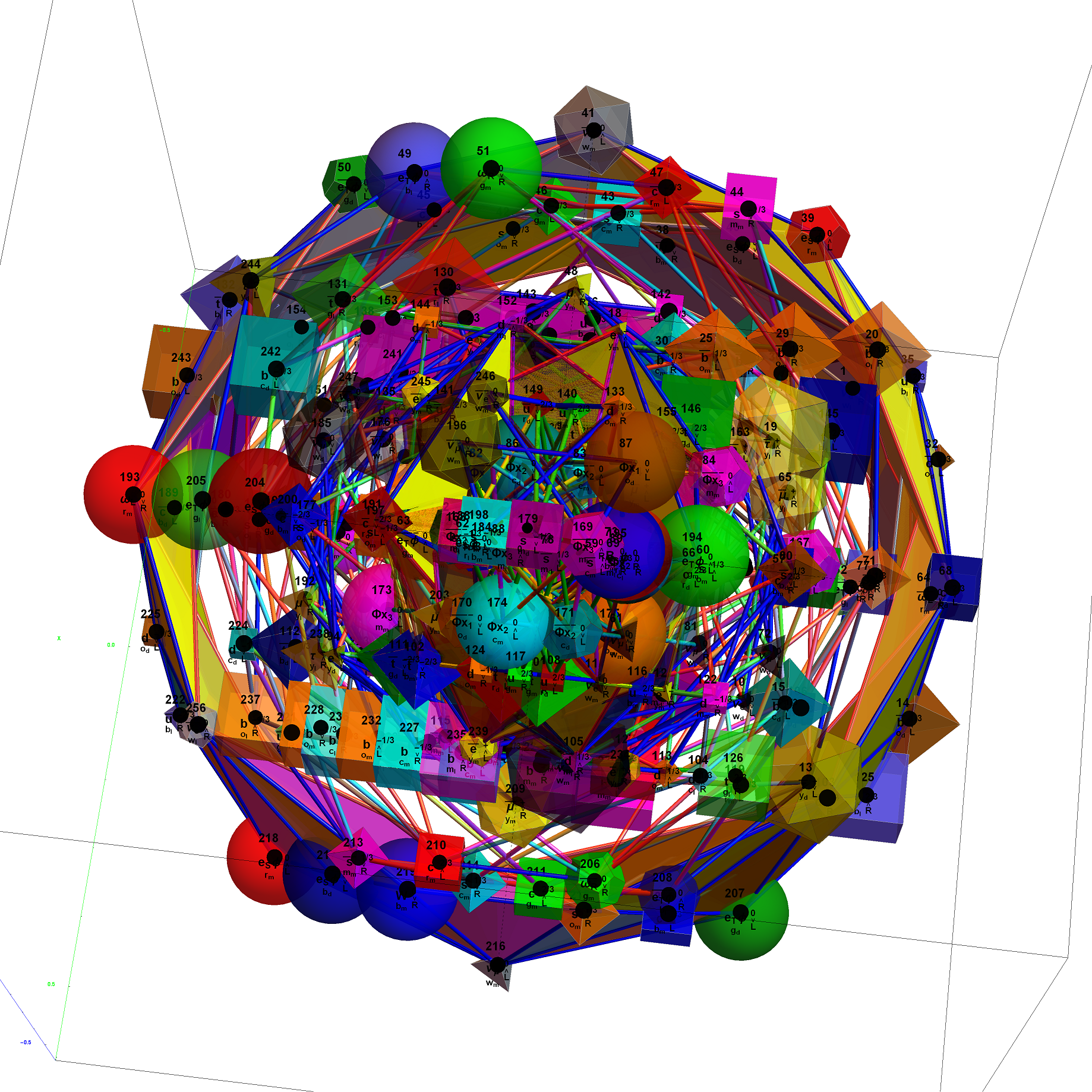
The 2^8=256 particles identify the known or predicted SM Fermions (192), Bosons (30 with 18 in the “Higgs Sector”), and the 8 dimension generator vertices (plus 8 excluded “anti-dimension” vertices). There are 18 remaining (Boson) particles added which are identified using an approach loosely connected with the theoretical work of A.G. Lisi in arxiv.org/pdf/0711.0770.
This approach to particle assignments allows for them to be associated with the 240 vertices of the split real even (SRE) E8 Lie group plus the 8 Orthoplex (dimensional) generator vertices (and 8 anti-dimensional generator vertices typically excluded from E8). The lexicographic ordering of the SRE E8 is consistent with a Cl(8) Clifford algebra, which has a familiar sequence of row 9 of the Pascal Triangle.
The particle families are split into 5 rows {two rows being the familiar 192 Fermion (l)eptons and (q)uarks, the 48 Bosons in the next two rows [Omega]g and [Phi][CapitalPhi], and a row for the 16 (Ex)ception dimension generator particles}. This demonstration applies a rigorous particle reference label for symbolic pattern matching to facilitate this identification. Each particle is given a unique 2D and 3D reference symbol. The symbol’s size, shape, color, and shade are used to uniquely identify the bitwise pattern. There are 2D particle shapes {circle, square, triangle} and their corresponding anti-shapes {pentagon, diamond, inverted triangle} and 3D shapes {sphere, cube, tetrahedron} and anti-3D shapes {dodecahedron, icosahedron, octahedron}. The particle’s SM generation alters the size in accordance to the tendency for mass to increase with increasing generation. The particle mass and lifetime (if known), are given by the ParticleData PDG curated data set for particles. The colors are, of course, used to identify the color content. The shade is modified with spin.
CKM:
See Neutrino Oscillations
There are added capabilities to view both the PNMN and CKM unitary triangle matrices, print and reference my ToE Neutrino mass predictions, which now accomodate the Koide relationships in particle masses.
Hadron:
See http://demonstrations.wolfram.com/CombiningQuarksIntoHadrons/
There are added capabilities to view the 4 and 6 Quark Hadrons as well as list all composite particles made up of the same quark content, including buttons to access their decay modes. To this list is a menu selectable Tooltip display of any particle property, and with decay modes shown with a button click.
See http://demonstrations.wolfram.com/HadronDecays/
This also integrates with particle selection on pane 3.
N-Body:
This demonstration combines several General Relativity (GR) / N-Body gravitational simulations across many space and time scales. There are configurations for asteroids and comets in our solar system, black holes centric galaxy formation, the origins of Large Scale Structure of the Universe, and Quantum Mechanics in Big Bang / Inflaton cosmology. At the top of the output pane is a LogLog Universal History plot with clickable Tooltips to select which epoch you want to simulate.
This simulation is incomplete.
Please note: The copy/paste of the Manipulate windows to .nb and .cdf don’t process OpenCL, so the Solar sim simply rotates the planets on their calculated orbital path and the other sims simply place particles randomly at each step (until I can fix it).
For Solar System related demos used (1),
See Cedric Voisin’s http://demonstrations.wolfram.com/LengthScalesInTheSolarSystem/
See Jeff Bryant’s http://demonstrations.wolfram.com/OrbitalElements/
See Enrique Zeleny’s http://demonstrations.wolfram.com/MercurysPerihelionPrecession/
See Andrew Moylan’s http://demonstrations.wolfram.com/TheFutureSolarSystem/
For Compton related demos used (4) ,
See Enrique Zeleny’s http://demonstrations.wolfram.com/ComptonEffect/
See S. M. Blinder’s http://demonstrations.wolfram.comKleinNishinaFormulaForComptonEffect/
ATOMic Elements:
A 2D/3D/4D (with s-p-d-f colors) Stowe-Janet-Scerri Periodic Table. This is organized by the four quantum numbers {n,l,m, and s=spin +/- 1/2}. The legend for how this maps to the traditional periodic table is shown to the right.
The isotope selection is not used with this UI. There is a selection for the n quantum number. In 2D display mode, this shows elements in the layer with that n quantum number. If in 3D mode, it will show all layers up to that selected n quantum number. As in the older version, a dropdown menu is available to show the detial element information in the tooltip. A slider for exploding the 3D display helps seperate the element layers. There is also a radio button to switch between the Stowe periodic table (Z=n) and the Scerri version (Z=n+l) when in 3D mode. Also available is a selectable option for showing the 2D/3D spherical harmonics of the Shroedinger electron probability density |[Psi],n,l,+/-m]|^2, based on whether it is in 2D or 3D display mode.
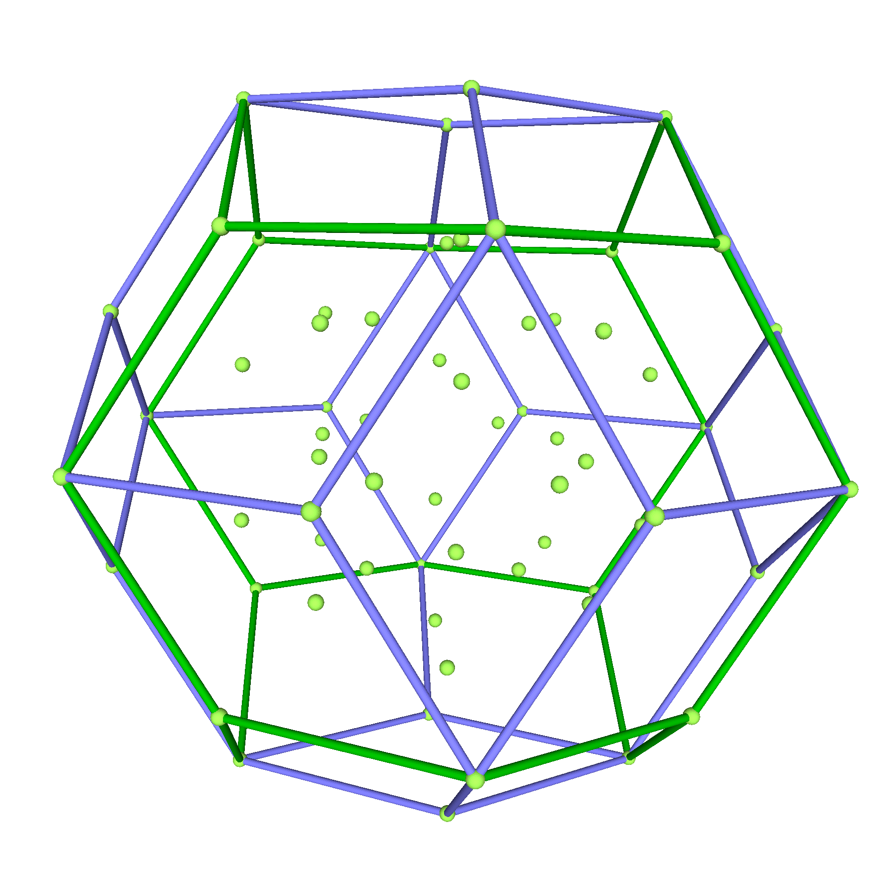
Interestingly, this periodic table has 120 elements, which is the number of vertices in the 600 Cell or the positive half of the 240 E8 roots. It is integrated into VisibLie_E8 so clicking on an element adds the particle who’s ordered E8 algebra root is that atomic element number. The negative roots can be thought of as “anti-elements”. The physics checkbox enables showing the associated 2D or 3D physics particle for each element.
See http://demonstrations.wolfram.com/AnAlternativePeriodicTable/
See http://demonstrations.wolfram.com/PropertiesOfTheElements/
See http://demonstrations.wolfram.com/HydrogenOrbitals/
See http://demonstrations.wolfram.com/SphericalHarmonics/
See http://en.wikipedia.org/wiki/Alternative_periodic_tables
HMI User Interface:
Added user controls for manipulating the third pane (VisibLie_E8) Lie Algebra particle projection viewer are provided in the top section, including:
* The artPrint checkbox allowing for higher resolution 2D images and cylinders (vs. lines) for edges/trialities/clicked vertex relationships.
* The dataSet dropdown menu allows for selection of multiple sets of coordinates, including binary, E8, Physics (rotated E8), and the 600 Cell.
* The limit checkbox allows the vertices to be shown at the edges of the frame bounding box rather than be off the page (enabling a “dimensionally rigorous” hyperbolic viewing).
* The pSize dropdown menu selects the variable size for the boson particles (tiny, small, medium large, huge).
* The zoom slider is an 10^+/-24 zoom capability (for non-E8 data sets).
* The particle scale slider allows all particles to be scaled (0 to 1).
* The ticks determines how many tick marks to show on each axis (0 to 50) given the frame size.
* The frame slider allows a fine grained zoom (0 to 2) determines the X,Y,Z bounding box (frame) dimension.
* The VisibLie_E8 also has checkboxes for the display of Symbols, Coordinates, Mass/Lifetimes,
An extensive set of controls in this main window include:
If working with the .NB version with full Mathematica license, several added controls are available:
File In (read) / Out (save). With full Mathematica license, the buttons to read in a saved inFile can be used. The “out to file” checkbox activates output (the “file out only” checkbox is for very large animations that need too much memory to display). The Dir button & filename (input field) and file type dropdown menu establish output filename. This also produces a < file > .m to record the configuration changes.
Checkboxes for optional displaying of:
* particle vertices (pVertices)
* clicked vertex edge relationships (clickVerts)
* parametric 3D surfaces (surfaces)
* triangle surface meshes (polygons)
* enabling perspective projection using the nD camera viewpoint slider below (perspective)
* vectors from the origin {0,0,0} to all vertices (pVectors)
* vertex color coding based on how many are overlapping that projected position (pLocations)
* measured particle mass and lifetime (pMassLife)
* 2D circle or 3D sphere unit boundary (perimeter)
Sliders for controlling of:
* n-Dimensional camera location (+/- 5) (nD camera)
* rectifications of particles (0 to 5) (rectify)
* change the number of dimensions used for edge calculations, e.g. for n-cube polytopes (1 to 8 ) (dim)
* selecting the gradient color set used for color coding the particles (0 to 51). Allows selection from the 50 Mathematica color gradients or 0=Lisi’s original or 51=my new 24 color gradients.
Note: pOverlaps overrides the colors.
Miscellaneous controls:
* clear clickVerts will clear the clicked vertices
* 2D Face select allows switching which of 3 unique (of 6 cubic) faces to display. This also impacts which H, V, Z projection vectors the dimension locators modify (they operate on the first two in the list).
* frame center and view point are two sets of 2D sliders plus a z-slider which control a 3D position, buttons for small and large incremental movement are also provided.
** frame center controls where the center of the frame is relative to the origin (the 3D camera points to this location)
** view point controls where the 3D camera position is in space.
* Norm’d edges ListPicker menu allows the selection of multiple sets of edges based on norm’d edge lengths {Value, Qty}. These change based on datasets and the number of edge dimensions (vertical dim slider).
* eFrames and eWindow sliders create animations of edges (the number of movie frames and the number of edges in each window – each calcuated based on how many edges are selected for display – starting with shortest projected inner edges).
* EdgeListAnimate checkbox will force an animation of all sets of Norm’d edges.
* The inner filter slider will filter out 0 to 100% of the selected edges (starting with shortest projected inner edges).
* eColorPos checkbox colors the edges based on their position in the projection as opposed to assignment based on their sequence in the edge list.
* eColors is a slider (like pColor) that selects the edge color gradient.
* scale surface is a slider to select how big the parametric surface objects are relative to the frame.
* surface color selects whether to apply edge color selections to the surfaces (vs. the default surface).
* eRadius is a slider (.001 to .1) that determines the diameter of the edge cylinder (3D w/artprint) or line (2D or w/o artprint).
Controls related to the particle filters:
Binary or bitwise particle filters:
* clear filters resets all 256 particles “optional” display property to “?”.
* OR / AND Logic radio button selects the type of binary logic to be applied to the selected binary filters. OR uses button-bars (allows combining of multiple elements of a binary set). AND uses radio buttons (only 1 selection per binary set)
* The “Row Filter” filters particle sets by the assigned rows in the ToE model (including Leptons, quarks, bosons (1 & 2), and/or excluded particles).
* Anti-Type-Color-Spin-Gen Filters are 1 or 2 bit binary sets associated with each particle parameter (anti, pType, color, spin, gen).
Note: Each of these sets defines the shape/color/shade/size of every particle.
pLists dropdown menu for selecting subsets of particles. Based on their anti-type-color-spin-generation properties, or Group Theory (S0{10},SO(8), E7,F4,G2,A2.”Favorite” projections.
Controls related to the vertex projections:
Viewing the static positions of particles by flying through the 8D space is done by projecting them (dot product) into a 2D or 3D view.
* reset Path resets all path settings back to original “Favorite” (aka. numeric other projections) selection.
* Translational/Rotational/Trans-Rot/Spin3D radio buttons select whether the chosen sliders will calculate an 8D rotational or translational path. Spin3D will simply rotate the 3D image around the Z axis.
* Identity/ptCoords radio buttons that select the type of beginning and ending flight path endpoint calculations:
** The 3 selected H,V,Z “Identity” vector is applied to the initial path point. Final path point is the current H,V,Z location indicators below.
** The 3 selected +/-H,V,Z “ptCoord” coordinate dimension indicators are applied to the initial and final identity dimensions path points.
* Favorites (aka. other projections) dropdown menu is used for selecting a growing set of favorite 8D H, V, Z projection vectors (by number, annotated in the full .CDF and .NB files).
* H,V,Z coordinate indicators/adjustors – for each H,V,Z Dim & Projection vector rows:
** Toggler Buttons select which of the 8 dimensions can be used in calculating rotational/translational paths and/or surface calculations.
** Vertical slider bars and numeric text fields can be used to adjust the value of the projections and endpoints for paths