https://fgmarcelis.wordpress.com
http://members.home.nl/fg.marcelis/
Really cool analysis of E8 geometry. I would love to collaborate, but can’t seem to find any contact info. If anyone knows him or can contact him, let me know.
I found his ’79-’81 Masters Thesis “Collectieve beweging in atoomkernen” from tue.nl
He co-authored a paper B. J. Verhaar, J. de Kam, A. M. Schulte, F. Marcelis: Simplified description of y vibrations in permanently deformed nuclei. Phys. Rev. C18 (1978) 523.
and see he participated in the HISPARC collaboration.
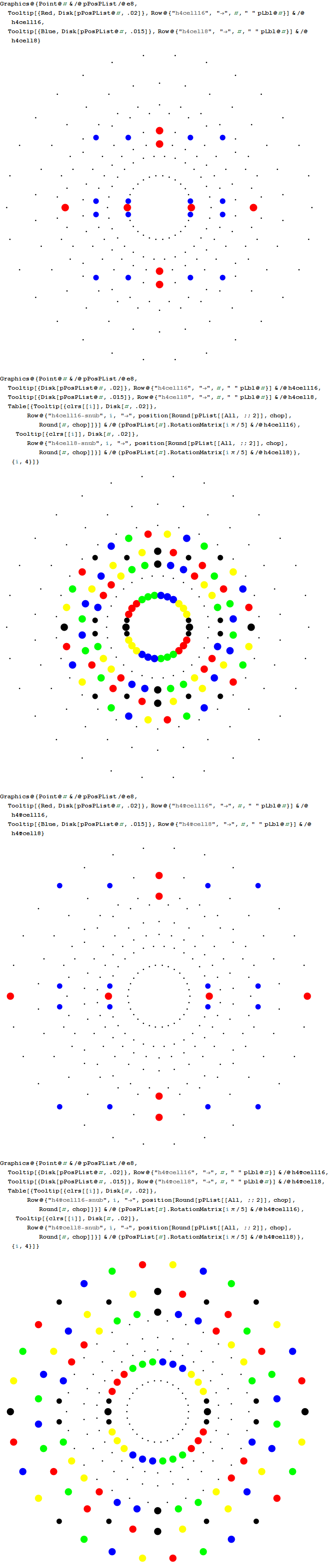
Some of my work that may support his is shown in this post, which shows how there are 10 self dual 24 cells in 2 sets of 5 (one for each H4 600 cell within E8). These are broken down by dual 16 vertex 8-cells and 8 vertex 16 cells. Marcelis creates a set of 14 8-cells (224 vertices) plus a basis of 16 vertices.
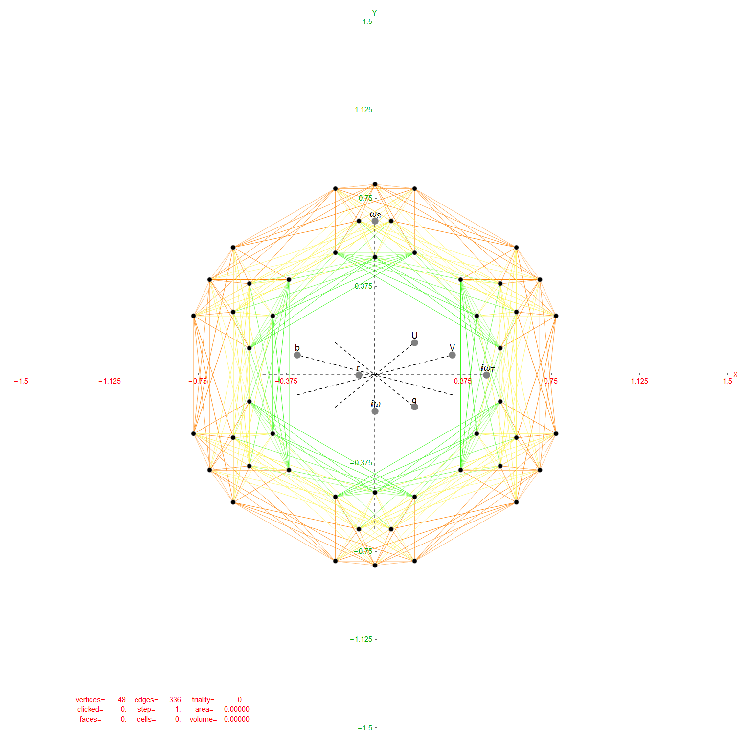
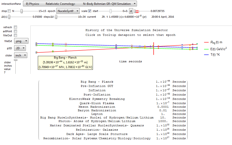
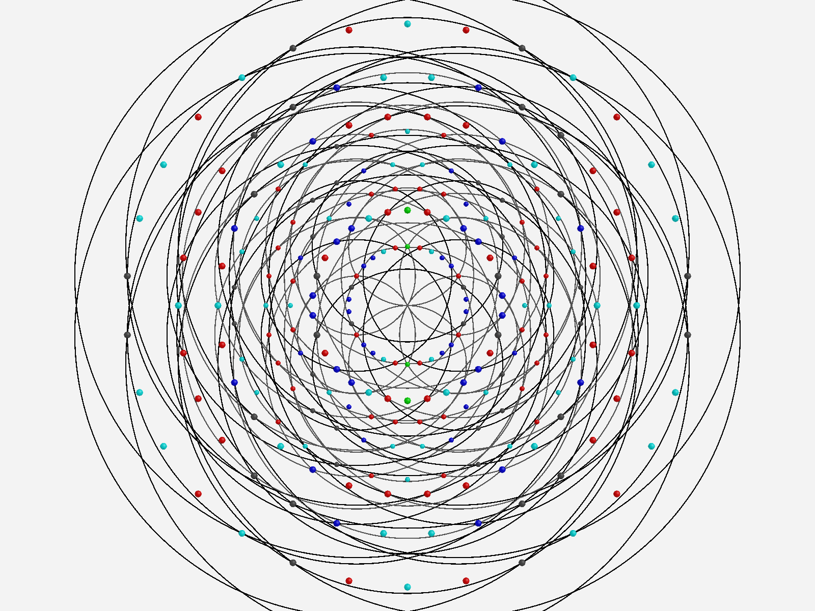
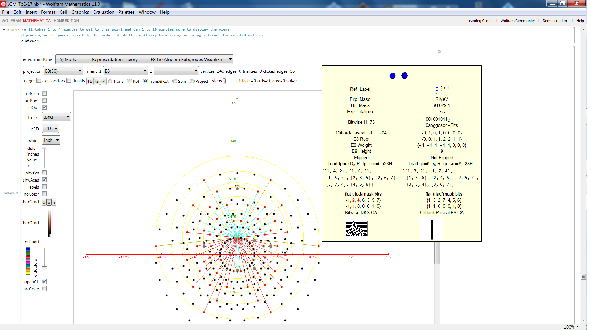
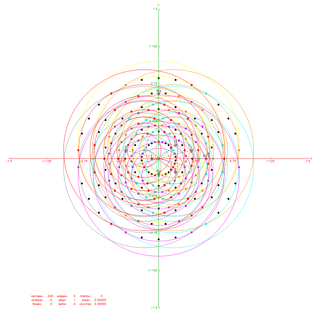
I replicate some of his work below using my Mathematica demonstration code as a base. When clicking a given vertex in my tool, it generates the edges to the 56 nearest vertices to that clicked vertex (as measured in all 8 dimensions). These are indeed the same vertices as those that intersect the rings of E8 Petrie Projection after translation to the clicked point.
Ring intersections that complement the 240 E8 vertices from 3{3}3{4}2. This is like clicking every 5th vertex (6) on the inner ring of E8 Petrie Projection.
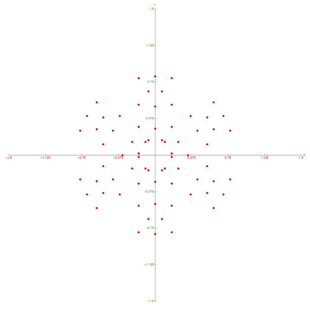
Vertices from 3{3}3{4}2
Inner 3{4}3
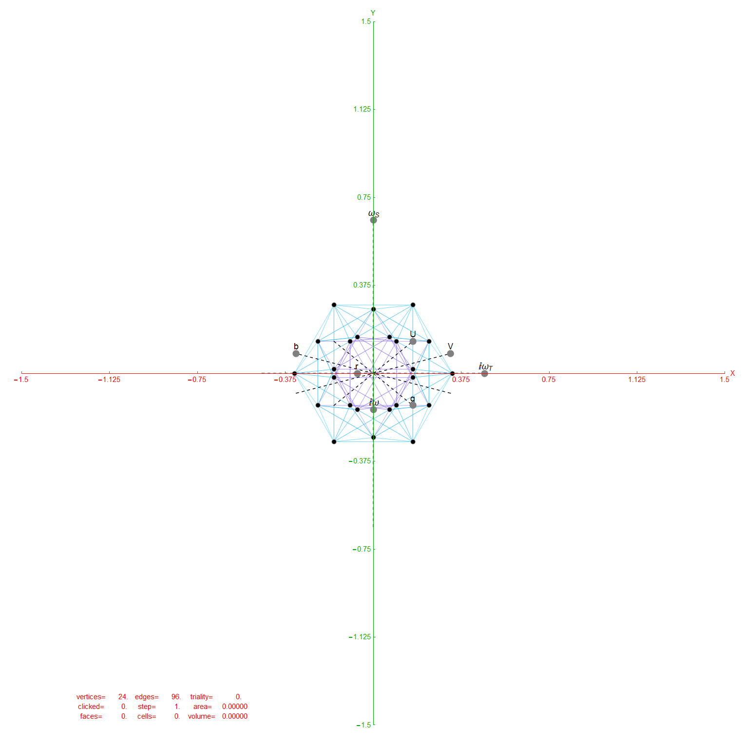
6 Outer 3{3}3