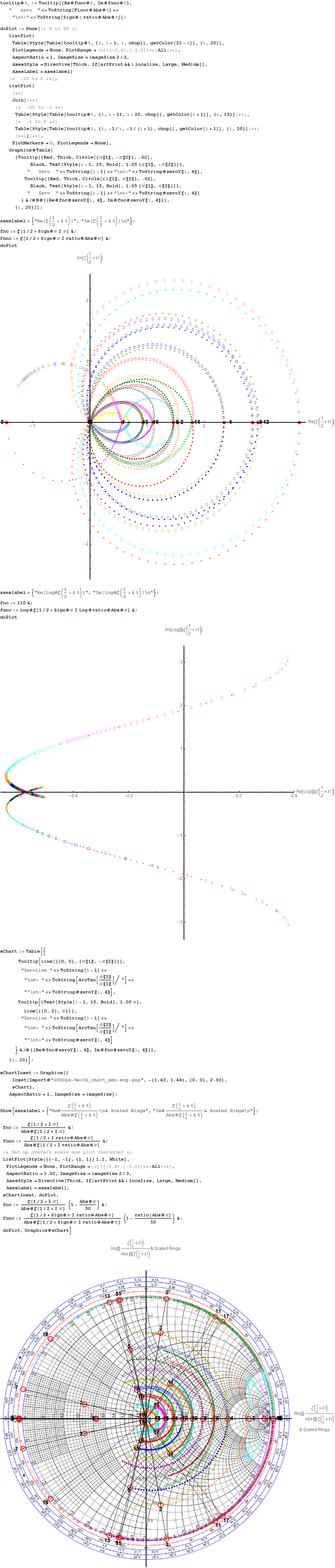
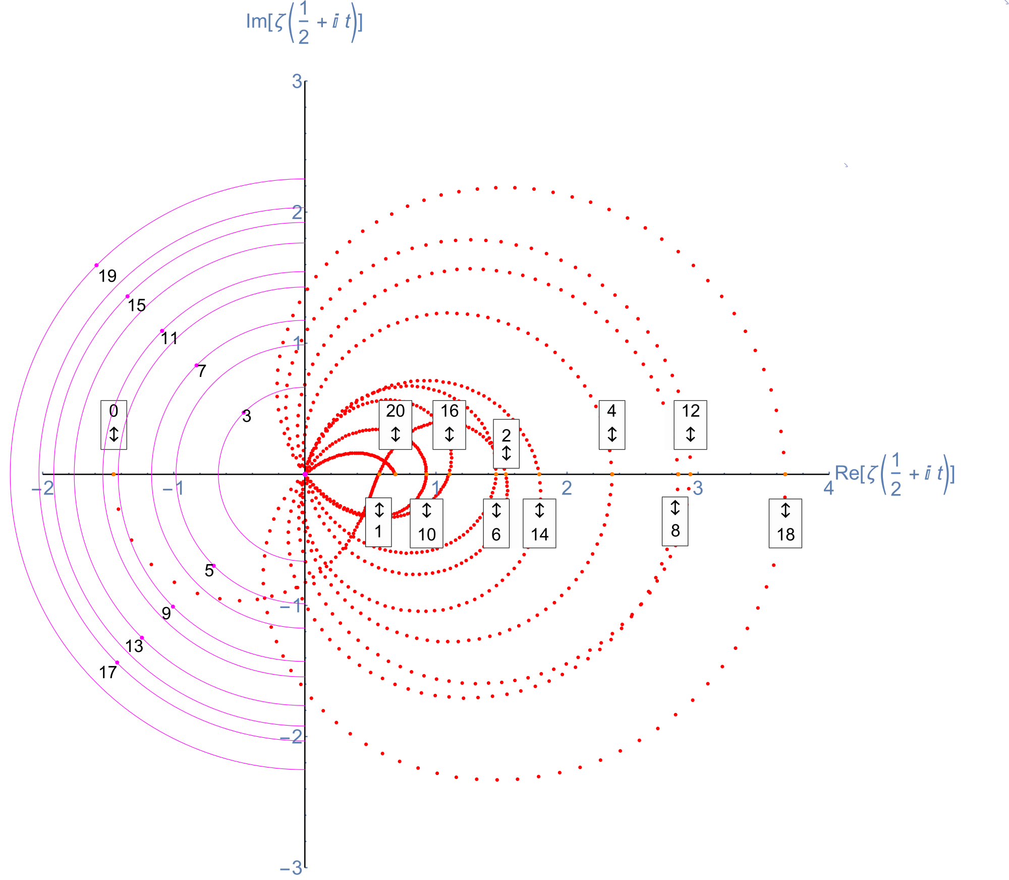
This web enabled demonstration shows a polar plot of the first 20 non-trivial Riemann zeta function zeros (including Gram points) along the critical line Zeta(1/2+it) for real values of t running from 0 to 50. The consecutively labeled zeros have 50 red plot points between each, with zeros identified by concentric magenta rings scaled to show the relative distance between their values of t. Gram’s law states that the curve usually crosses the real axis once between zeros.
A downloadable copy is available ZetaZeros-local-art-50.cdf Latest: 05/23/2016.
Note: The interactive CDF plug-in as required below does not currently work on Chrome browsers.
A Snapshot picture for those w/o Wolfram CDF interactivity:
Selectable example code snippet:
[wlcode]Show[ListPlot[Style[pts2, Red], PlotRange -> {{-2, 4}, {-3, 3}},
AspectRatio -> 1, ImageSize -> imageSize,
AxesStyle ->
Directive[Thick, If[artPrint && ! localize, Large, Medium]],
Graphics[{PointSize@.01,
tttxt := If[artPrint && ! localize, tttxt1, ttxt0];
If[ttxt0 = ToString[# – 1];
Abs@zeroY[[#, 1]] < 10 chop,
(* Magenta Critical Line Zeta Zeros *)
tttxt1 =
Column[{ToString[# - 1], "t=" <> ToString@zeroY[[#, 4]]},
Center];
ttLoc =
zeroY[[#, 4]] If[artPrint && ! localize, 1, 2] imagesize/40000;
(* Flip Point Labels above/below the X axis *)
ttLoc1 = {-1, (-1)^Round[#/2]} ttLoc/Sqrt[2];
{Magenta, Point@ttLoc1,
Circle[zeroY[[#, ;; 2]], ttLoc, {1, 3} \[Pi]/2],
Black,
Tooltip[Text[
Style[tttxt, If[artPrint && ! localize, Large, Medium, Bold]],
(* Shift the Labels off the Point *)
ttLoc1 (1 – (-1)^Round[#/2] .05)], tttxt1]},
(* Orange Critical Line Imaginary zeros w/Real>0 *)
tttxt1 =
Column[{ToString[# – 1], “x=” <> ToString@zeroY[[#, 1]],
“t=” <> ToString@zeroY[[#, 4]]}, Center];
{Tooltip[{Orange, Point@zeroY[[#, ;; 2]], Text[Style[
Column[If[EvenQ[Round[(# – 1)/2]], Prepend,
Append][{“\[UpDownArrow]”}, tttxt], Center,
Frame -> True],
Black, If[artPrint && ! localize, Large, Medium],
Background -> White],
(* Flip Point Labels above/below the X axis *)
zeroY[[#, ;; 2]] + {0, (-1)^Round[(# – 1)/2]} If[
artPrint && ! localize, 1,
If[artPrint, 4/1, 3]] imagesize/5000]},
Column[{ToString[# – 1], “x=” <> ToString@zeroY[[#, 1]],
“t=” <> ToString@zeroY[[#, 4]]}, Center]]}] & /@
Range@Length@zeroY,
Magenta, Disk[{0, 0}, .03]}]][/wlcode]
More plots with various scaling functions and multi-color coding along with Tooltip on mouse-over. Bear in mind the last Smith Chart with a division by Abs@Zeta indicates where the increments go exponential near the 0.
A Snapshot picture for those w/o Wolfram CDF interactivity: