Please see the latest in .nb, .cdf demonstrations files and web interactive pages.
| ToE_Demonstration-Lite.cdf | Latest: 08/15/2016 (10 Mb). This is a lite version of the full Mathematica version 11 demonstration in .CDF below (or as an interactive-Lite web page) (4 Mb). It only loads the first 8 panes and the last UI pane which doesn’t require the larger file and load times. It requires the free Mathematica CDF plugin.
This version of the ToE_Demonstration-Lite.nb (13 Mb) is the same as CDF except it includes file I/O capability not available in the free CDF player. This requires a full Mathematica license. |
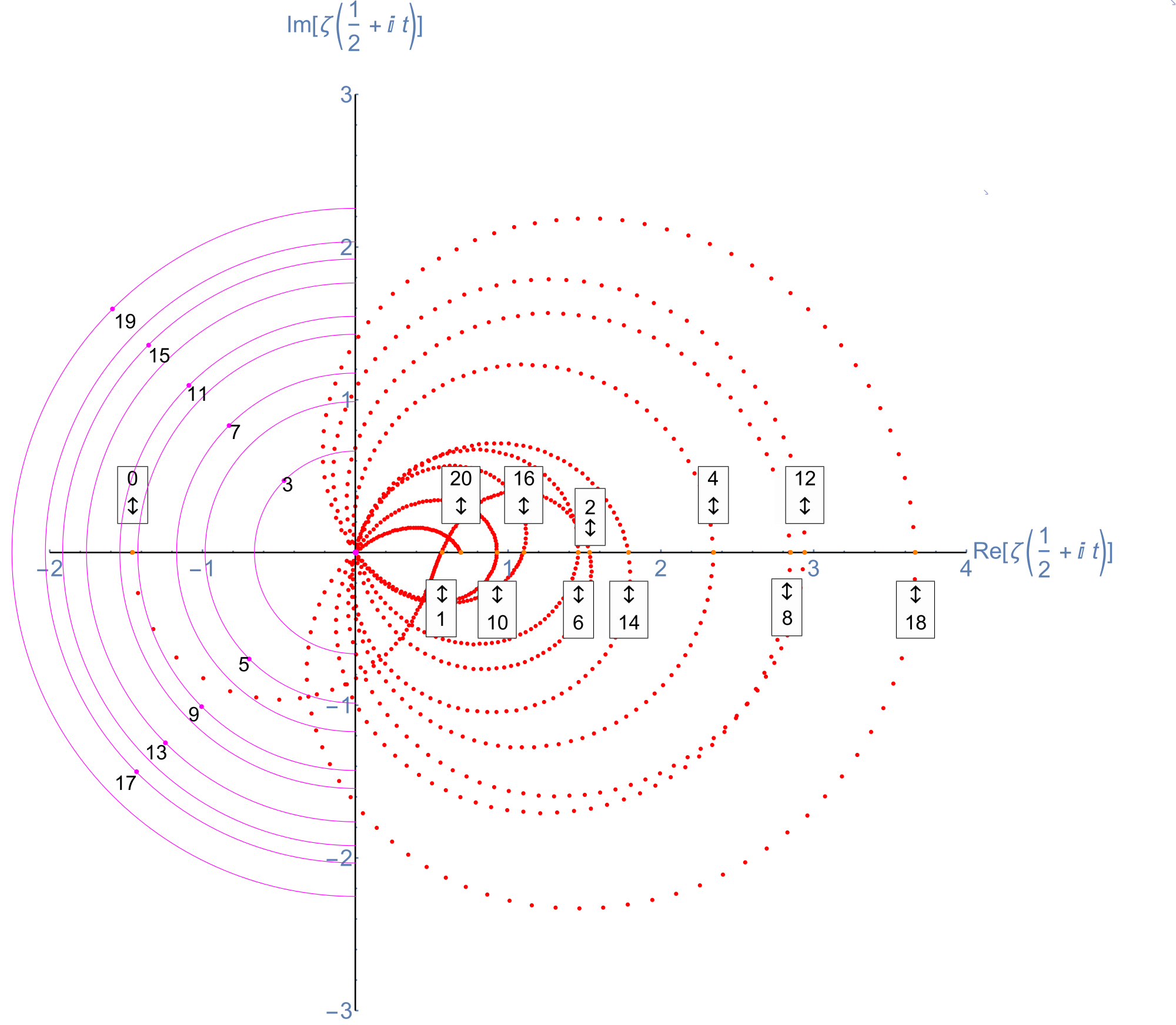
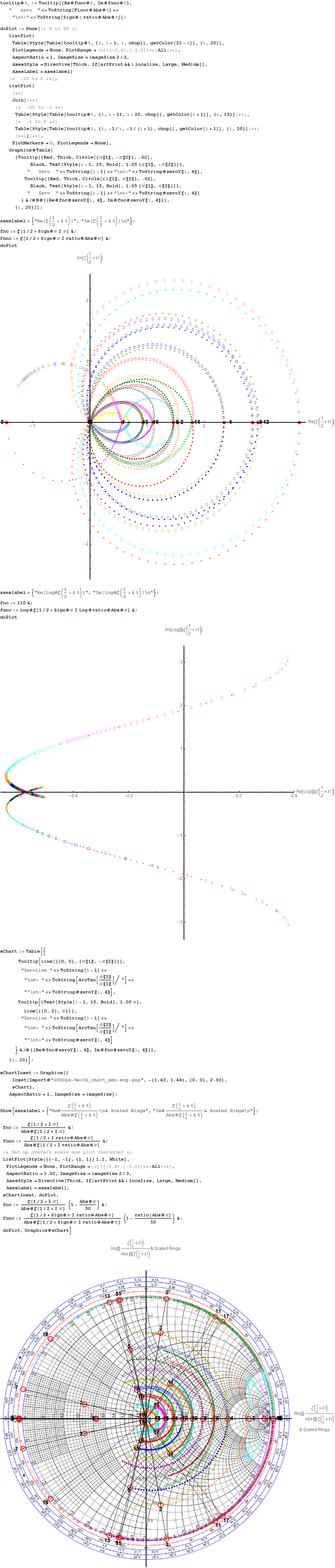
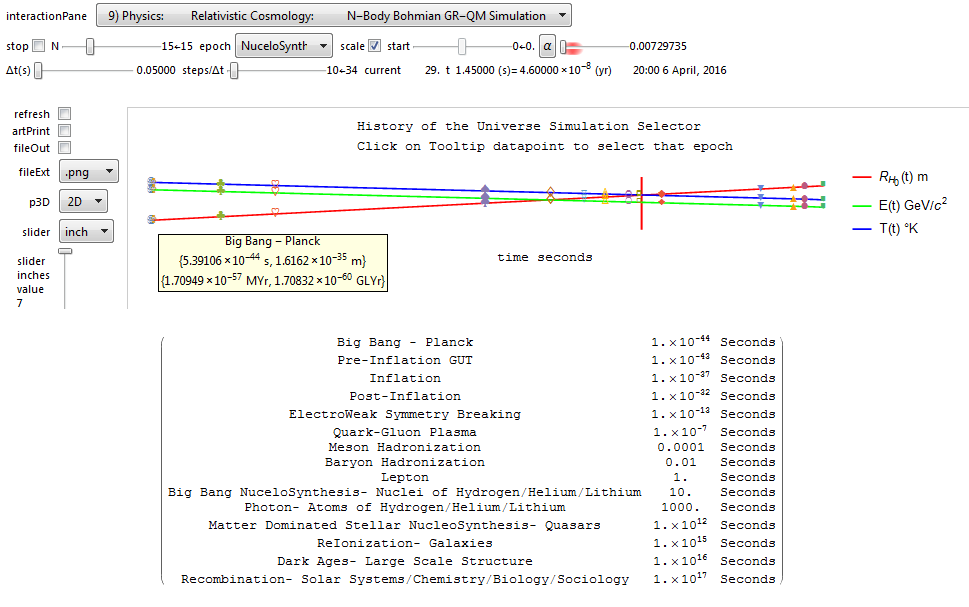
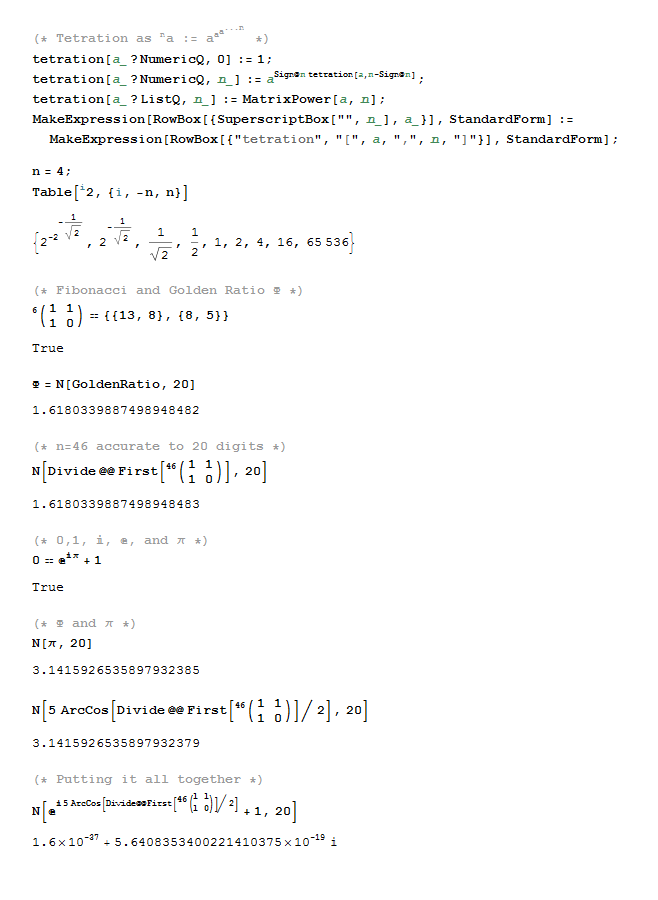
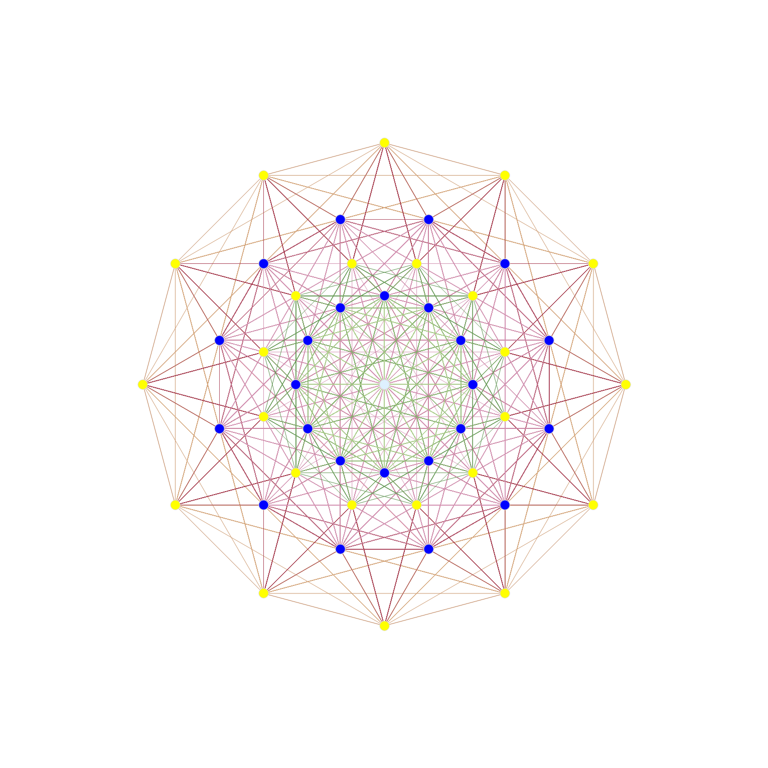
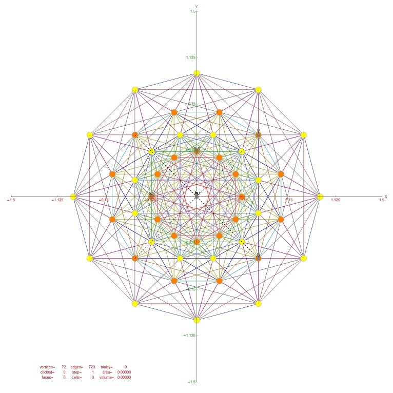
| ToE_Demonstration.cdf | Latest: 08/15/2016 (110 Mb). This is a Mathematica version 11 demonstration in .CDF (or as an interactive web page) (130 Mb) takes you on an integrated visual journey from the abstract elements of hyper-dimensional geometry, algebra, particle and nuclear physics, Computational Fluid Dynamics (CFD) in Chaos Theory and Fractals, quantum relativistic cosmological N-Body simulations, and on to the atomic elements of chemistry (visualized as a 4D periodic table arranged by quantum numbers). It requires the free Mathematica CDF plugin.
This version of the ToE_Demonstration.nb (140 Mb) is the same as CDF except it includes file I/O capability not available in the free CDF player. This requires a full Mathematica license. |
(The CDF player from Wolfram.com is still at v. 10.4.1, so still exhibits the bug I discovered related to clipping planes/slicing of 3D models).
