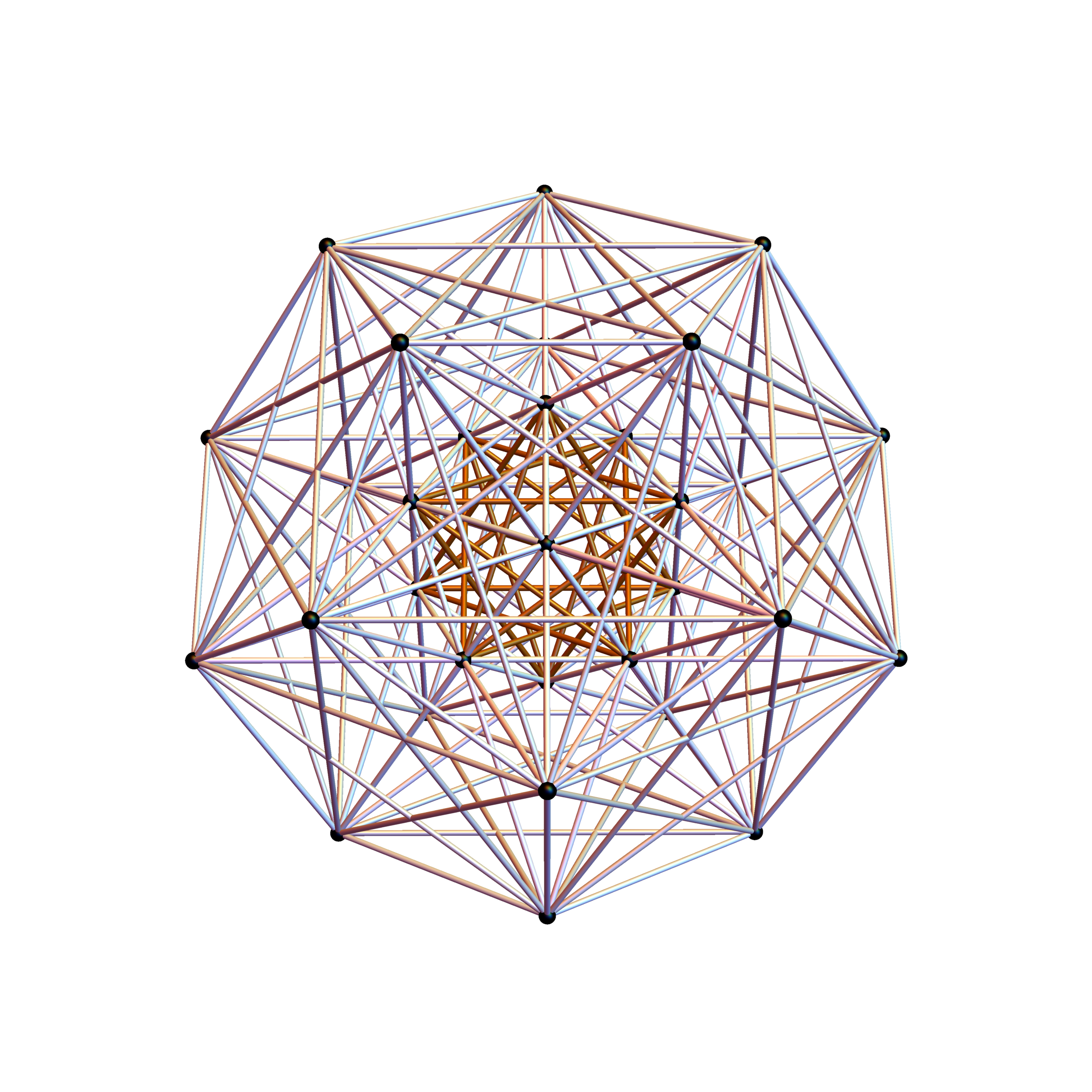
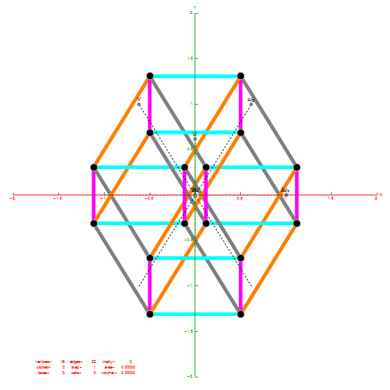
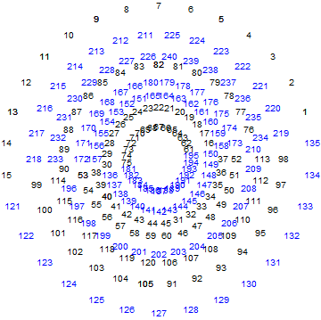
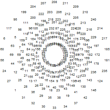
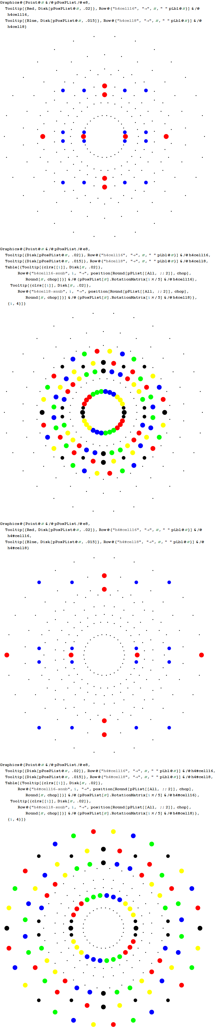
Below is an animated .GIF (3 seconds per frame) in 2D of E8 in Petrie projection with numbered vertices. It cycles between the full E8 (Gosset polytope), to the 8 16-Cell (Cross polytope) vertices, to the 16 8-Cell (Tesseract) vertices. It then cycles through the 5 H4+H4Φ 600-Cell pairs of 24-Cells (main 24-Cell and 4 Snub 24-Cells rotated around the Petrie projection).

Notice that 4 of the 8 16-Cell vertices are co-located on the axes with the basis vectors of the 2D projection. The other 4 basis vectors (on the right half of the 8D basis) are located at the origin {0,0}.

BTW – if you find this information useful, or provide any portion of it to others, PLEASE make sure you cite this post. If you feel a blog post citation would not be an acceptable form for academic research papers, I would be glad to clean it up and put it into LaTex format in order to provide it to arXiv (with your academic sponsorship) or Vixra. Just send me a note at:  jgmoxness@theoryofeverthing.org. 

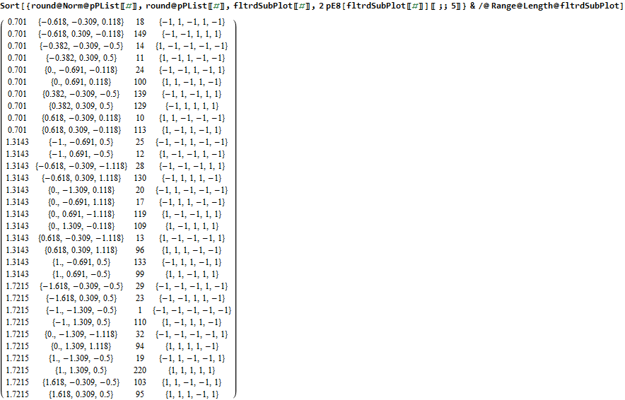
The Split Real Even (SRE) E8 vertices are numbered in order of their canonical sort position in the Pascal Triangle binary order. See the large .PNG graphic at the bottom of this post for the full list of binary, E8 and folded H4+H4Φ in symbolic and numeric values. The connection between E8 and the binary (binomial expansion) of the Pascal Triangle (Clifford Algebra) is visualized here. It is interesting to note that the binary and E8 vertex values of 1-128 are mirrored by the 256-129 (note: reverse order, with 0<->1 for binary or negation for E8).

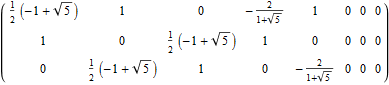
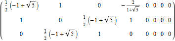
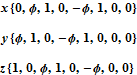
The H4 numeric and symbolic information is obtained through E8 vertex dot product with the 8×8 rotation matrix and is multiplied by 2 for clarity. H4 Folding is obtained by only using the top or bottom 4 rows of that matrix I discovered in 2010 (below):

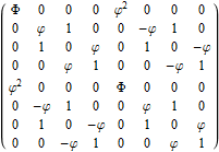
Notice the Quaternion to Octonion Cayley-Dickson like doubling procedure pattern in the 4 quadrants of this matrix. It is this pattern that is responsible for maintaining the 4 sets of 600-Cell H4 vertices when rotating from E8 vertices.

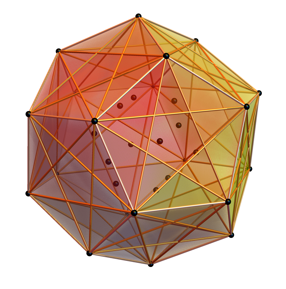
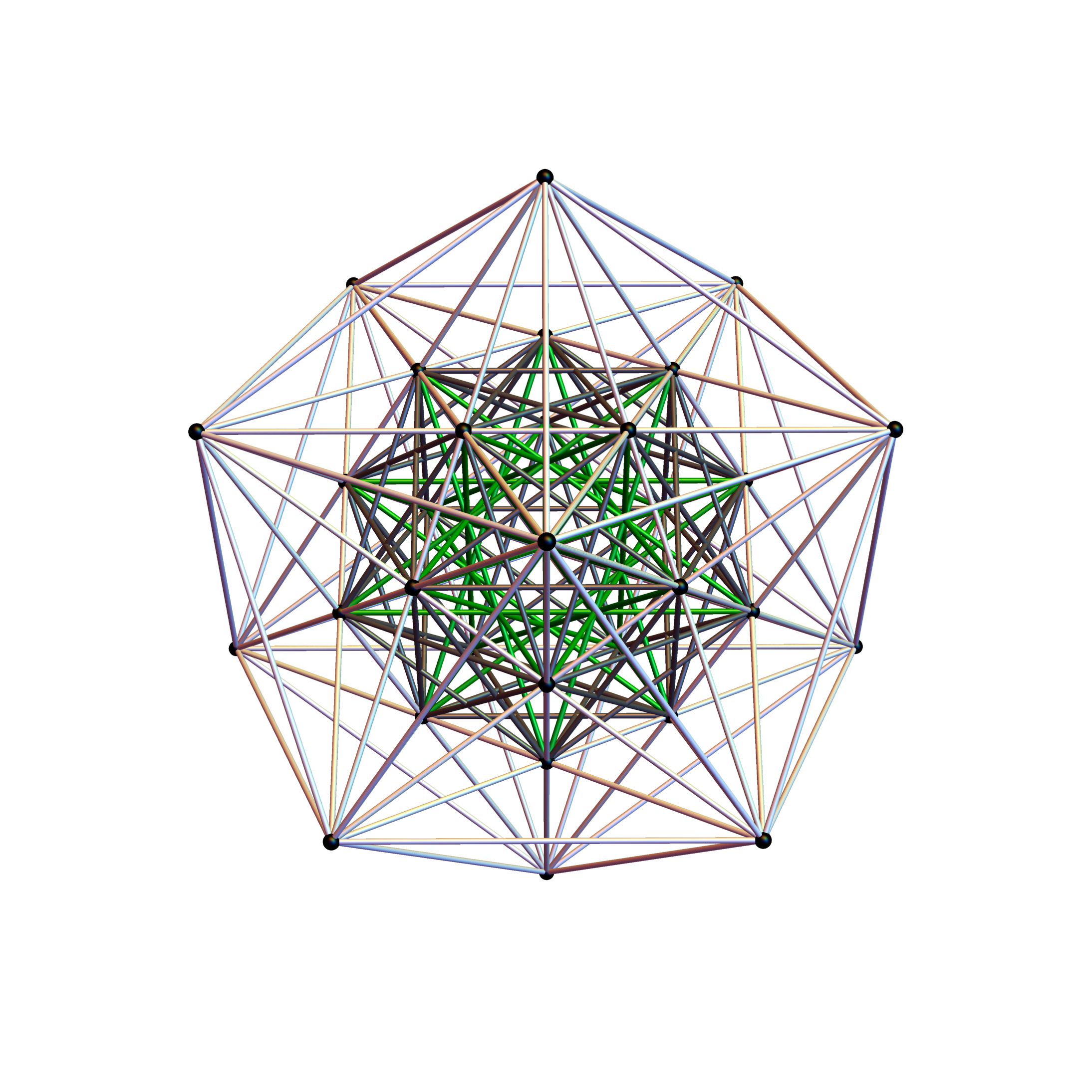
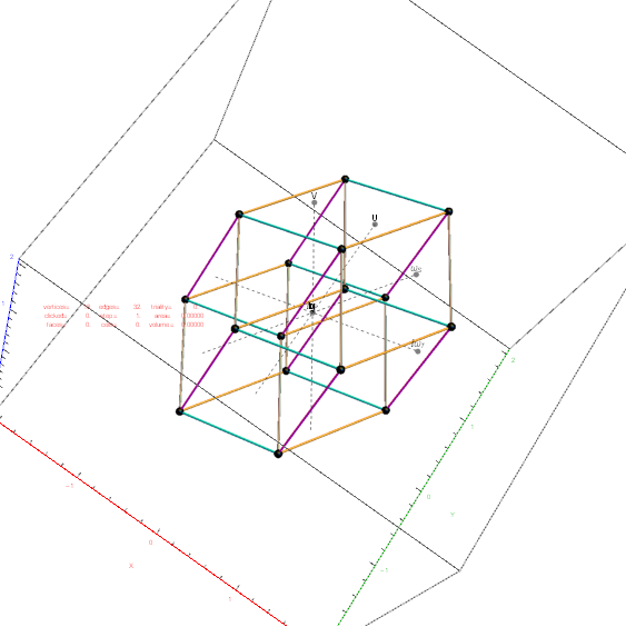
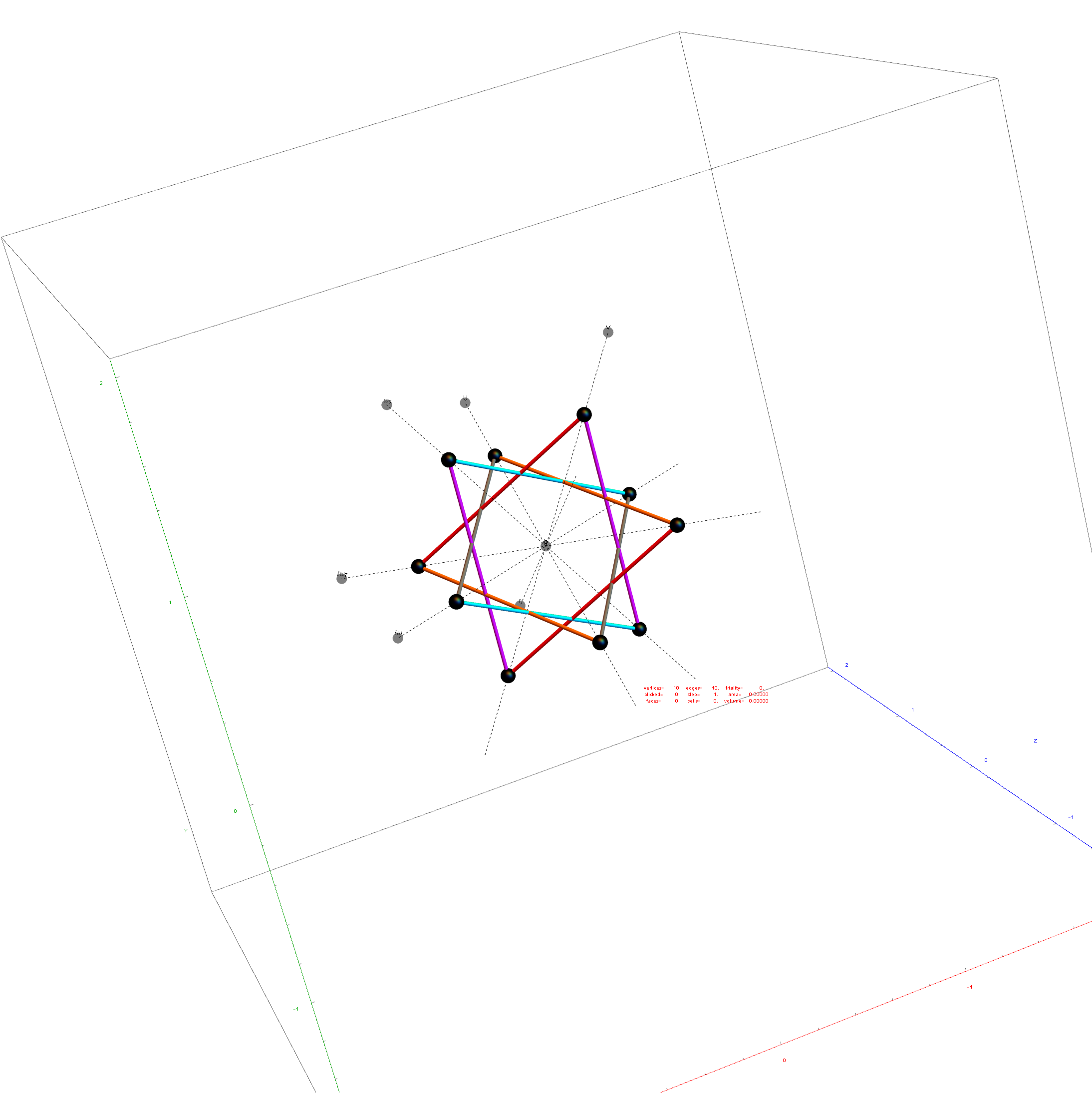
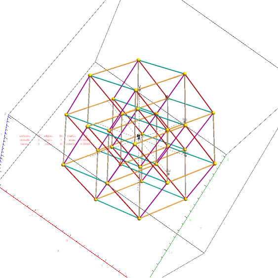
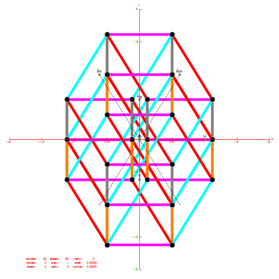
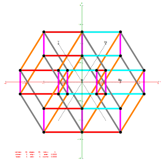
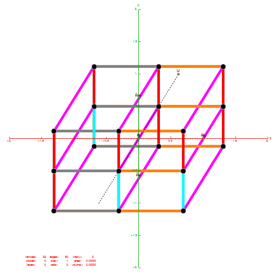
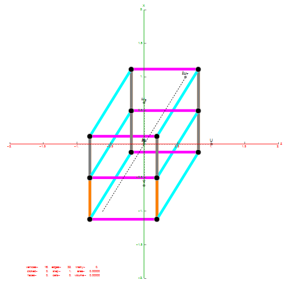
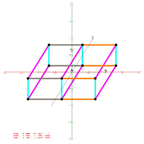
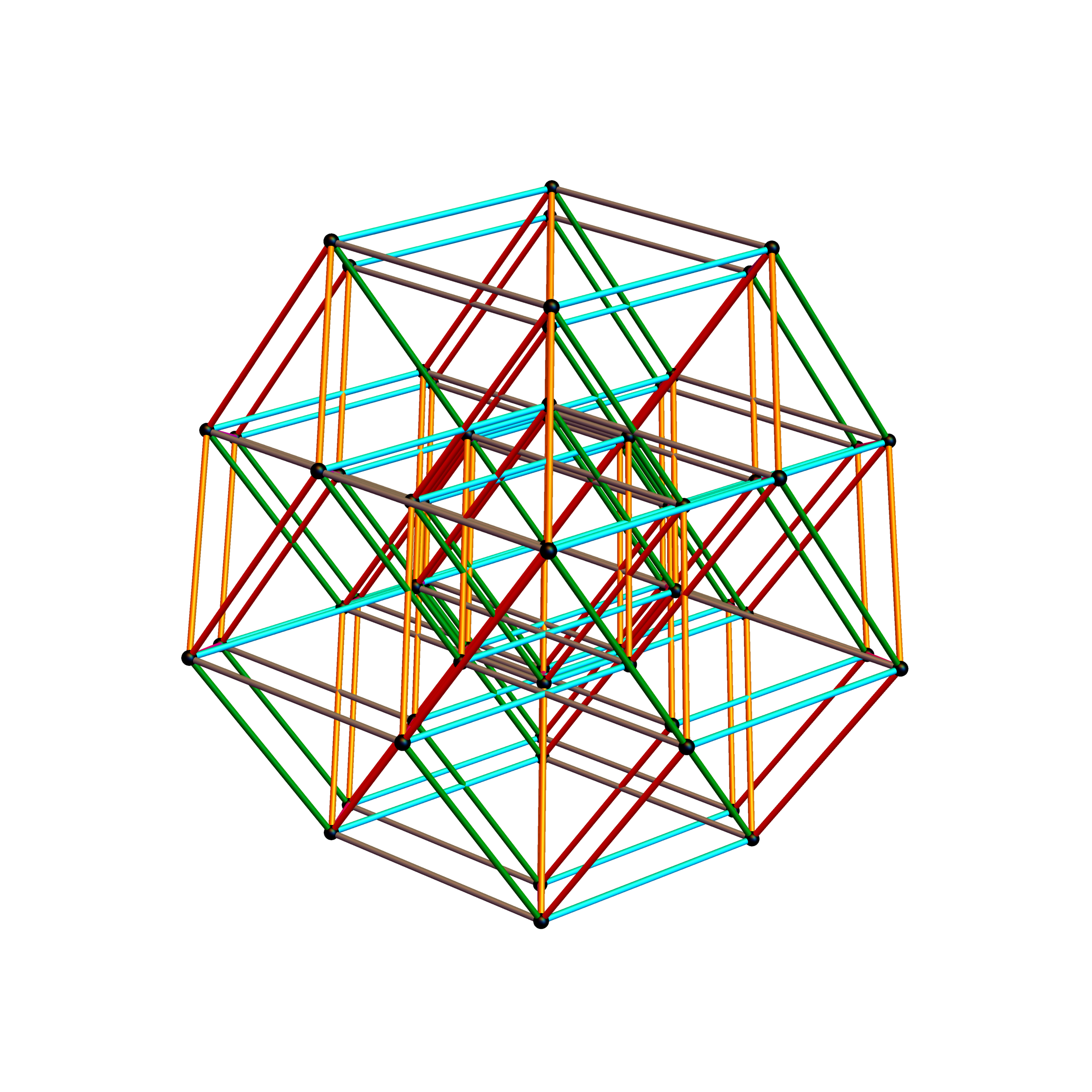
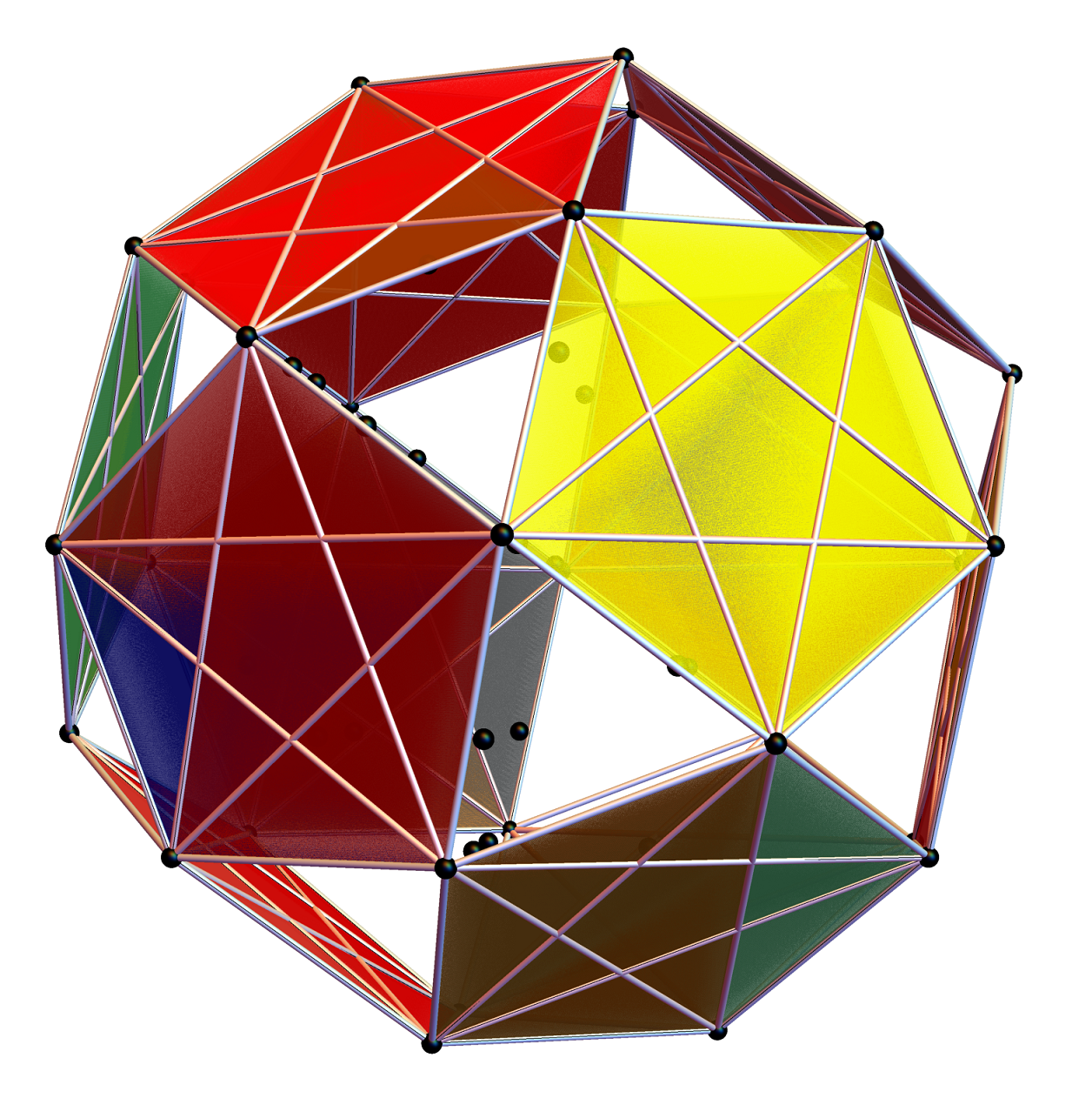
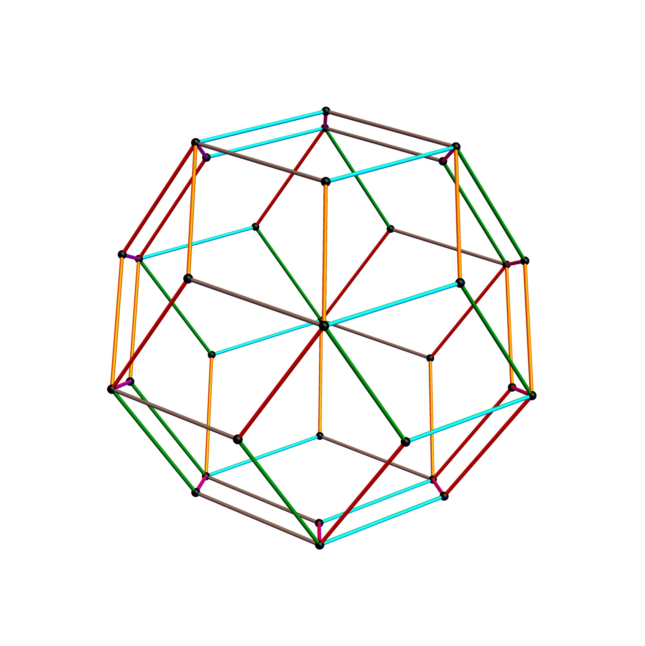
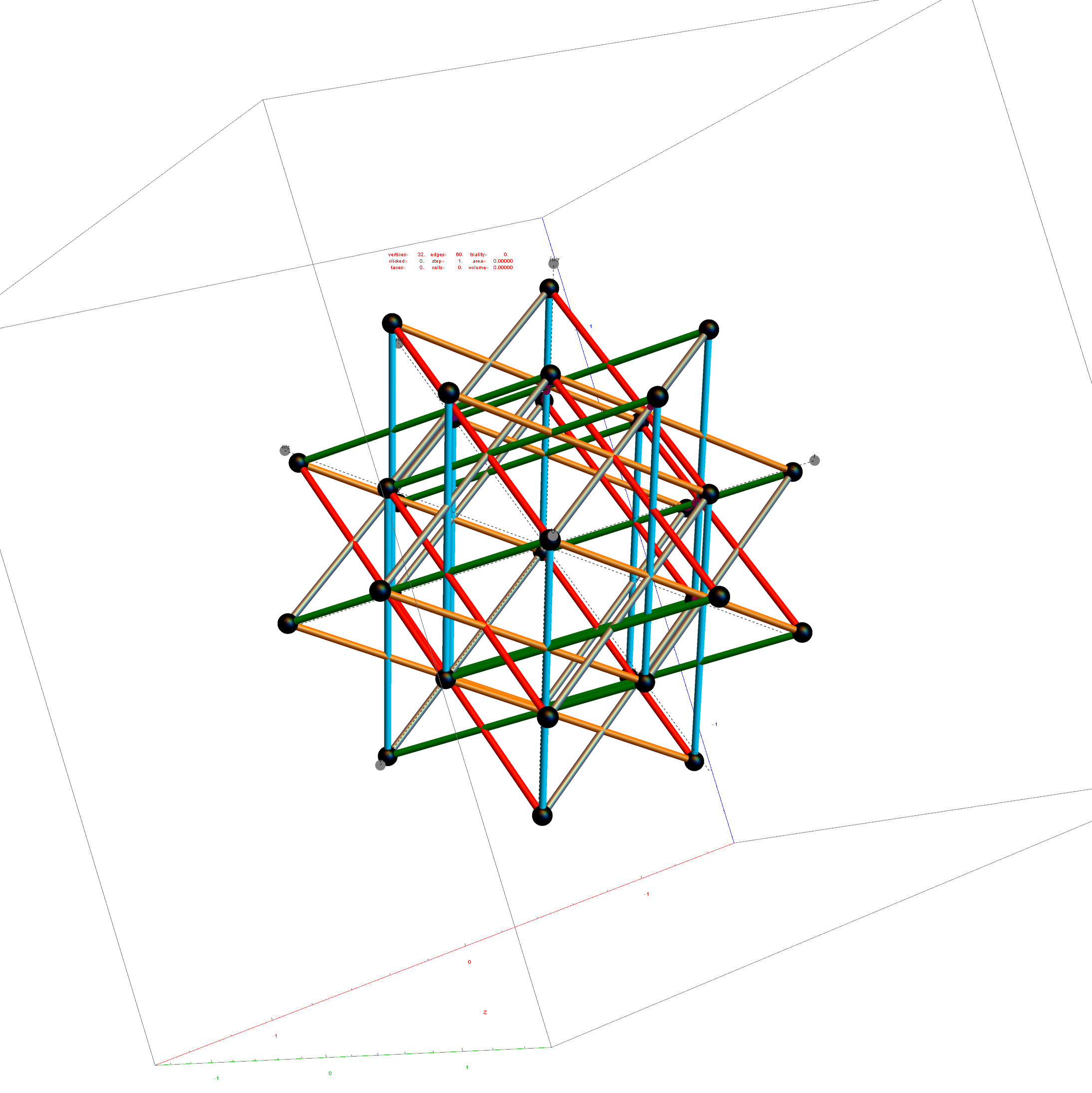
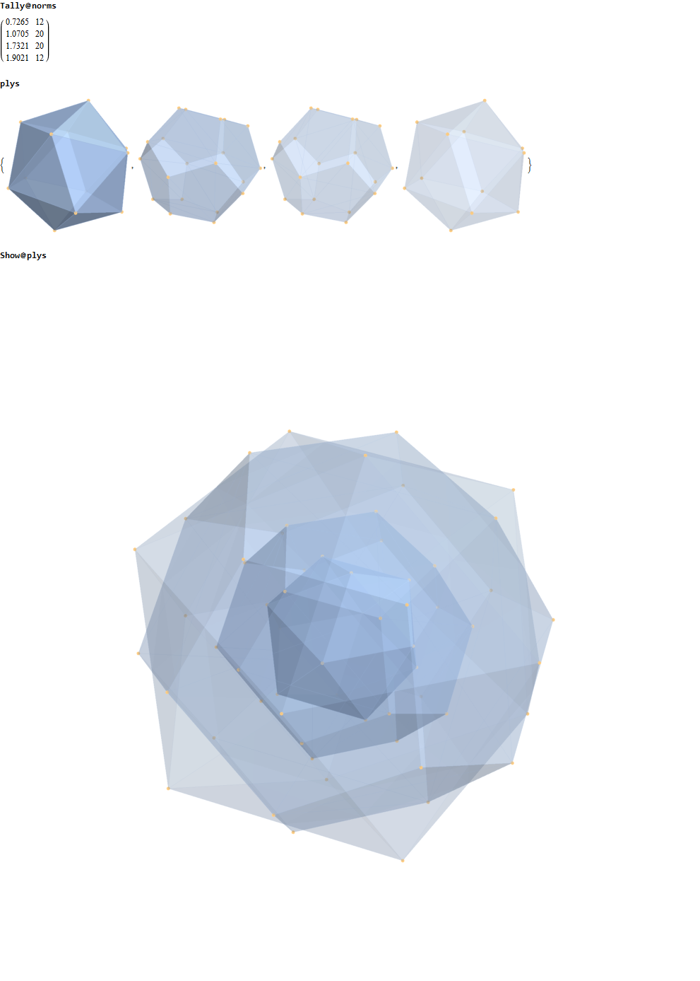
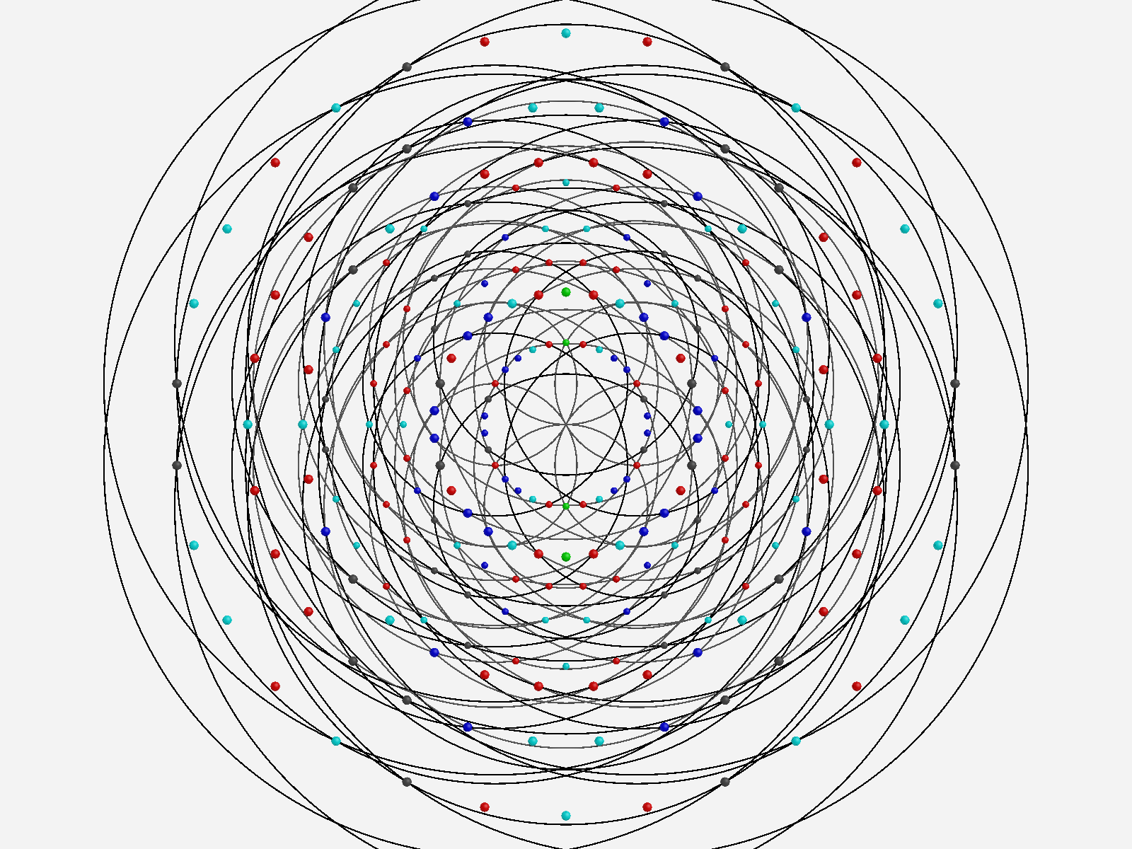
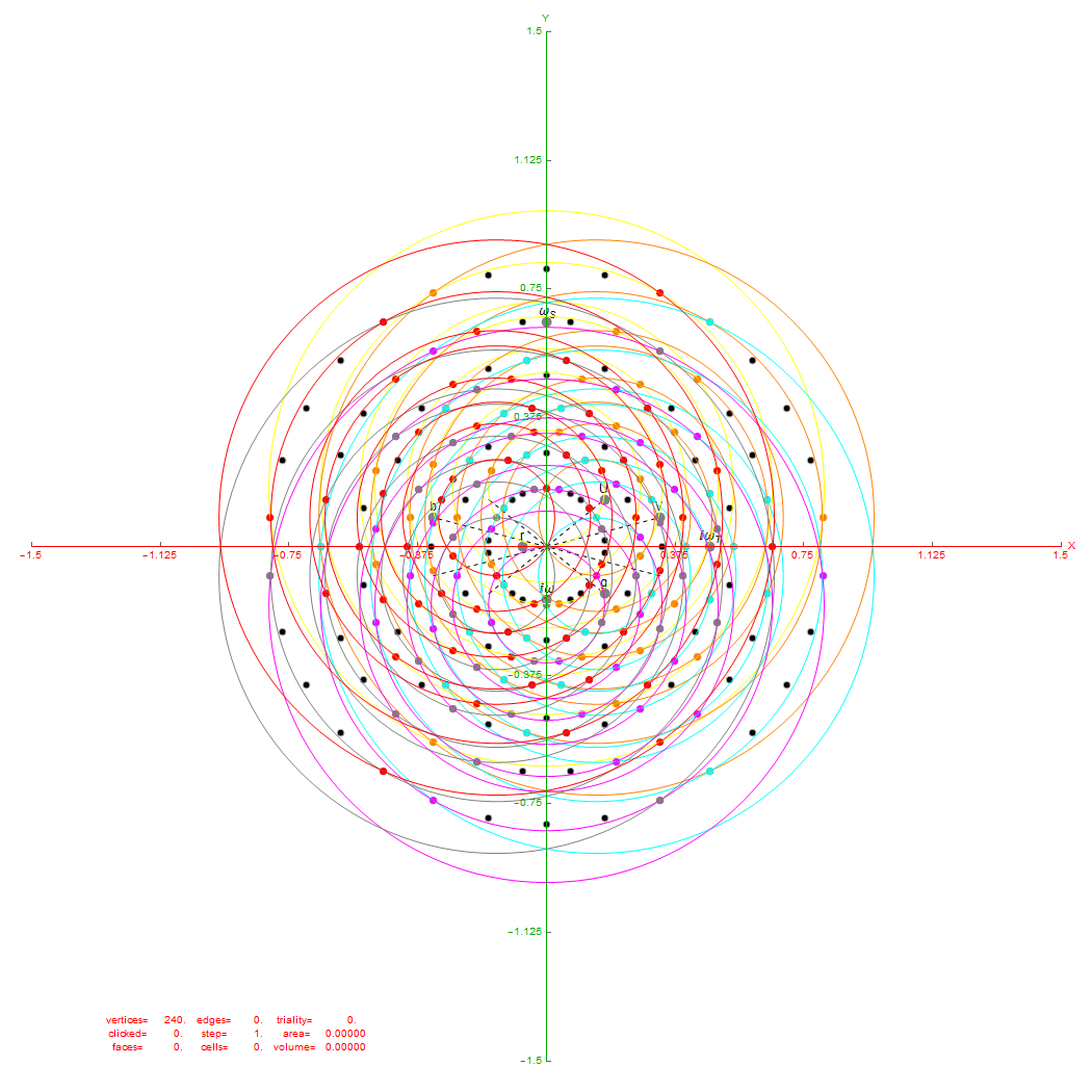
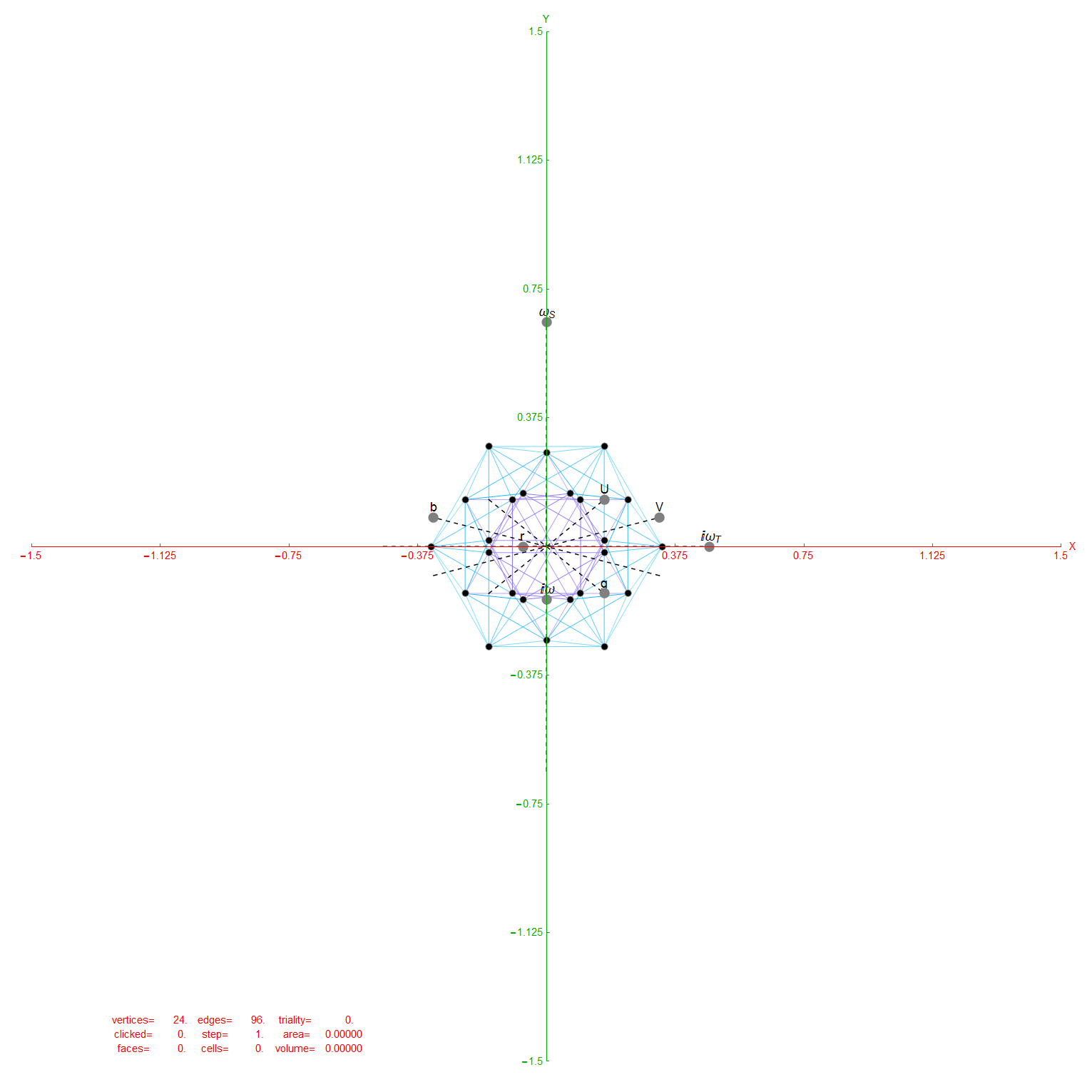
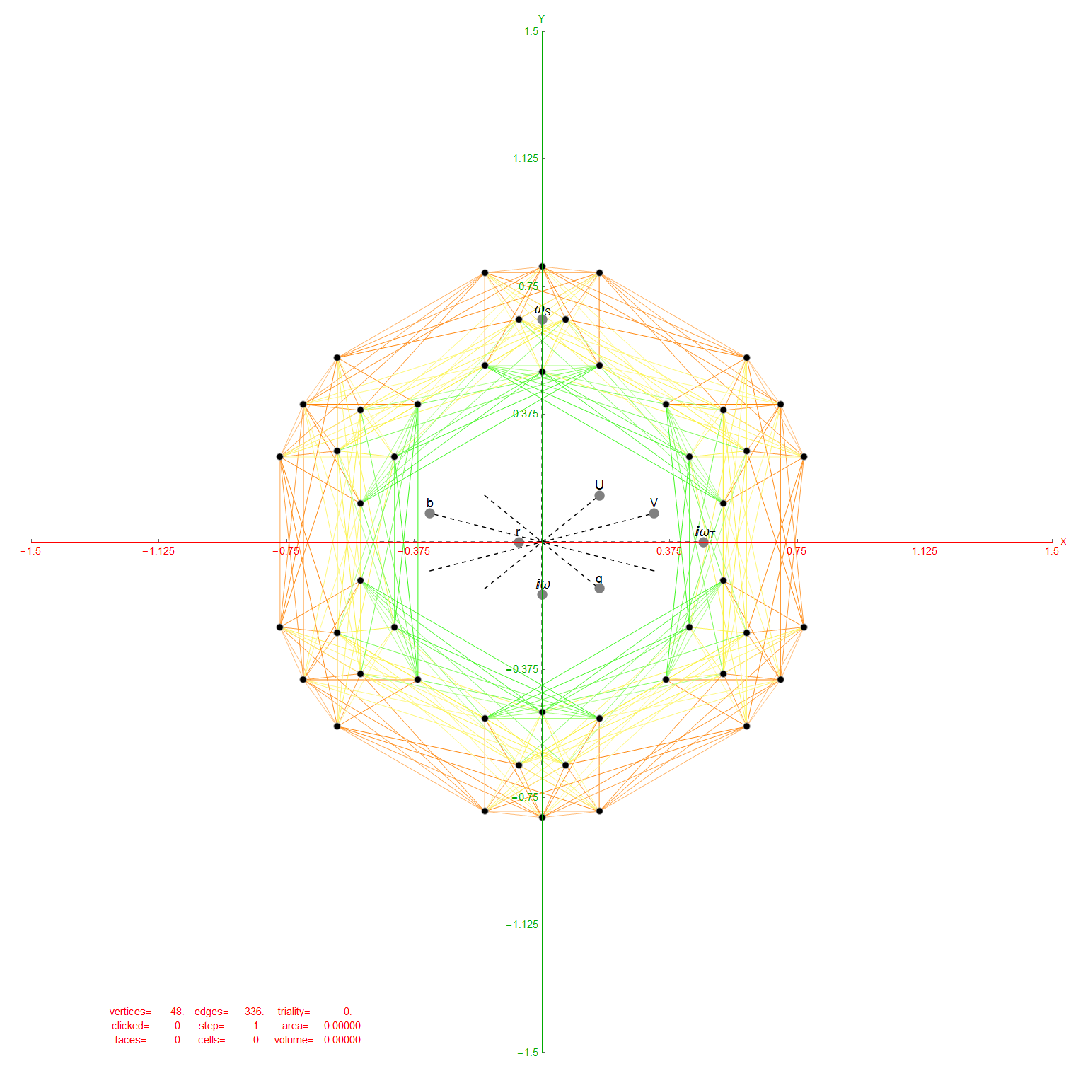
Below is the same type of animated .GIF from above, except it is projected into 3D by adding a 3rd basis vector for the z axis. These are shown without vertex numbers for clarity. It starts with E8 with 6720 8D Norm=Sqrt[2] edges (or equivalently E8 rotated to H4+H4Φ edges with 3360 4D Norm=1 & 3360 4D Norm=Φ edges). It cycles through to the H4Φ 600-Cell, H4 600-Cell, and then to the 24-Cell without edges. Finally on to the 8-Cell and 5 pairs of 24-Cells with edges. Again, the right 4D half of the 8D projection basis vectors are located at {0,0,0}. Of the other 4 basis vectors, 2 are on {x,y,z} axes.

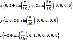
The projections of E8 rotated to H4+H4Φ in this post are not a pure ortho-normal 600-Cell projection, in that it is intended to show the Petrie projection on one face {x,y}. It does show the ortho-normal 600-Cell structure on another face {y,z} (albeit rotated off axis), and something in-between these on the {x,z} face. The full ortho-normal 600-Cell can easily be projected to full 3D symmetry on all 6 faces by using an ortho-normal basis. The 3 projection basis vectors used here in this post are as follows:

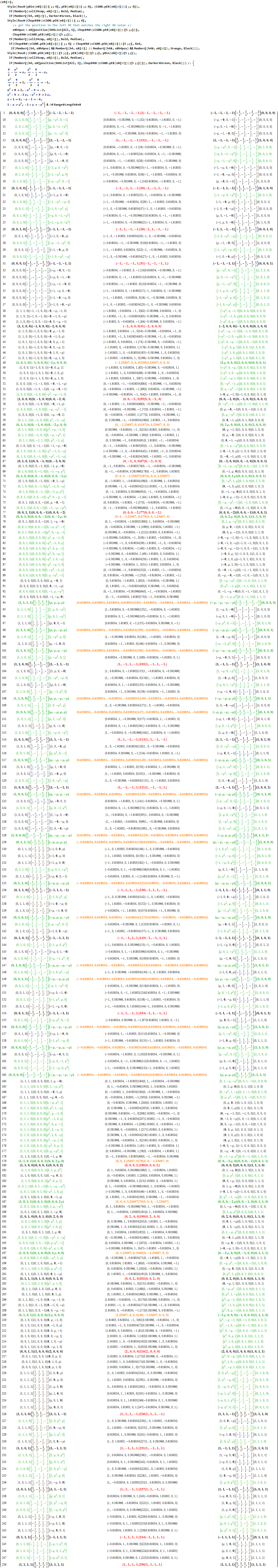
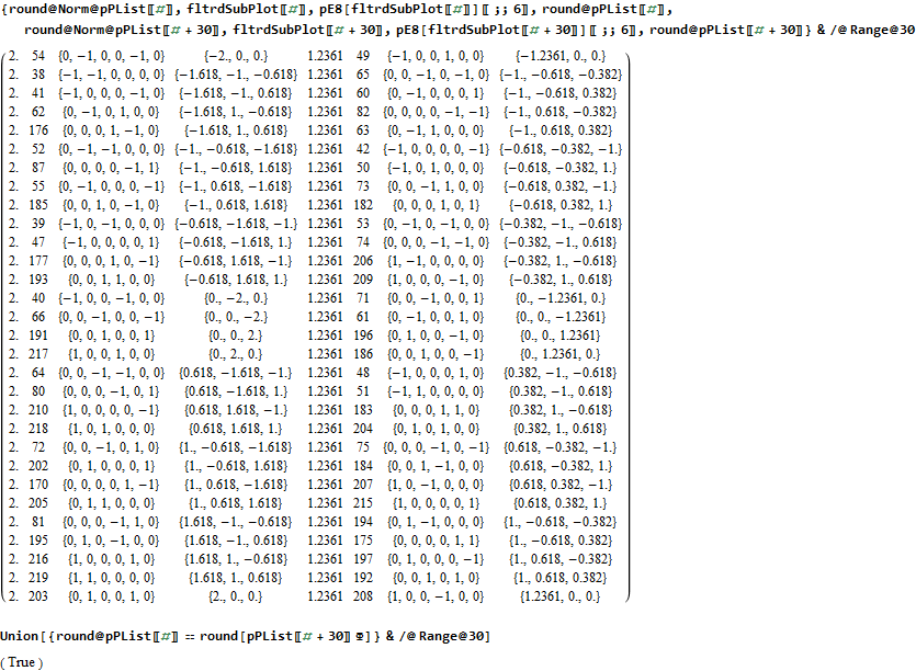
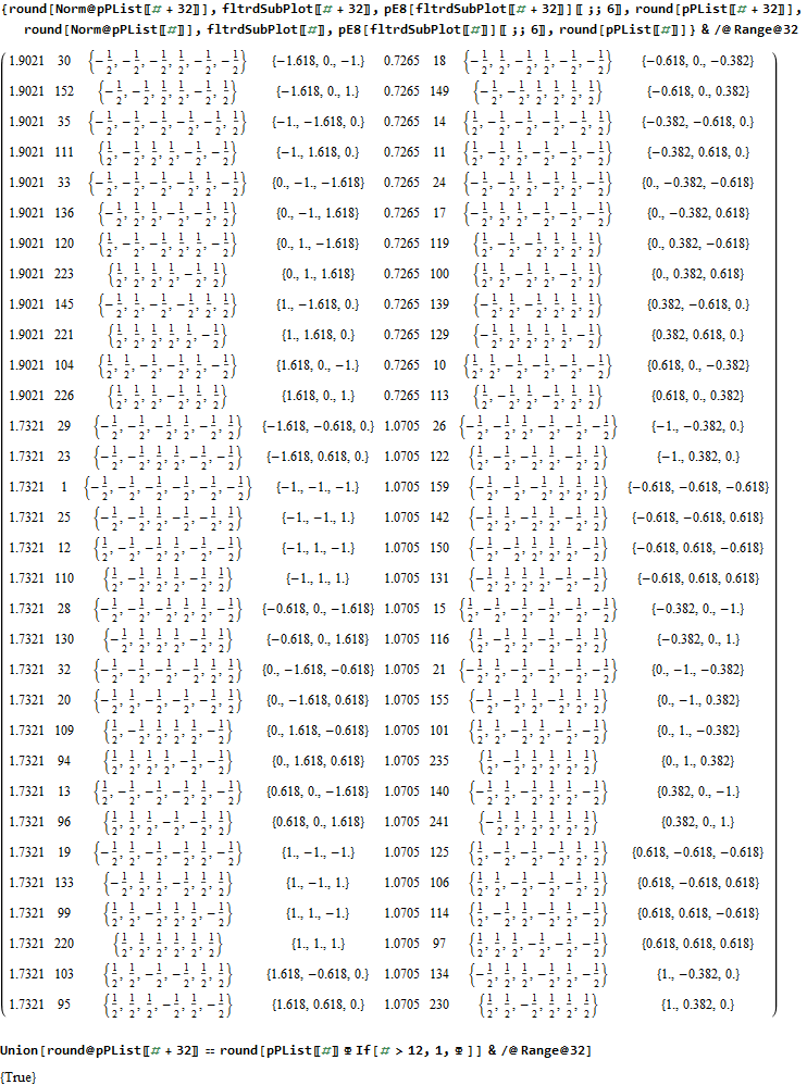
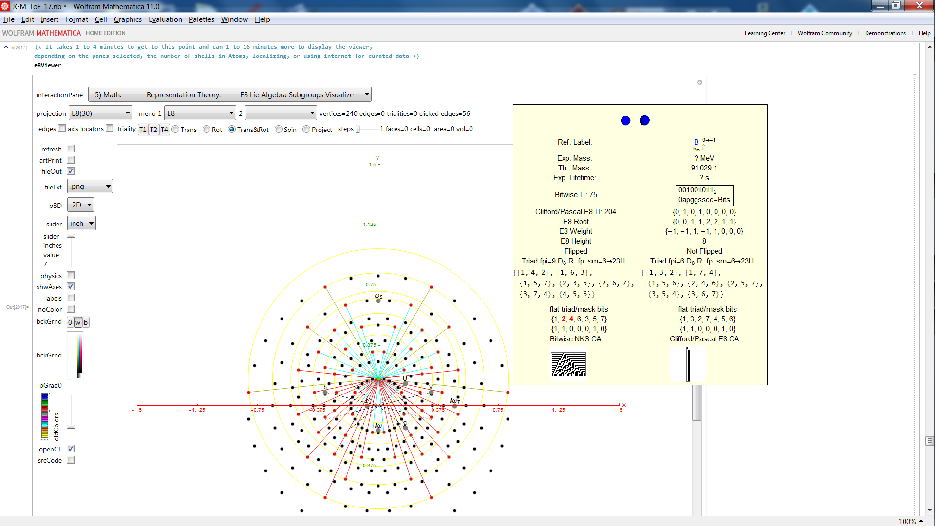
Below is the very long .PNG graphic listing the left 4D and right 4D vertex information for E8 (Pascal Triangle Binary and Split Real Even E8) and folded H4 and H4Φ in symbolic and numeric form. On the left side is the vertex number. Notice vertices 2-9 and 248-255 are missing. These are the 8 generator (and anti-generator) E8 vertices. The center of each row is a number that identifies the vertex where the left and right 4D elements switch sides to right and left.

The green data in the left and right columns indicate a 4D H4 vertex, while black in those columns indicate H4Φ 4D vertex. As you can see, there are actually 4 H4 600-Cell constructs in this E8 rotation, with 2 on the left and 2 on the right.

Wow – that is nice! Remember, you heard it here first!

The red text in the center column indicates vertices of the H4Φ 24-Cell. Notice, all the red vertices don’t switch left/right since they have symmetric 4D halves. Interestingly, 1/2 of the 16 H4Φ 8-Cell vertices are made up of 1/2 of the 16 8-bit Hamming (distance 4) binary codes. The other 1/2 of those Hamming codes are located in the 16 H4 8-Cell vertices, with anti-symmetric left/right halves (described in the next paragraph).

The Orange is the H4 24-Cell. While this 24-Cell does have a different vertex identified in the center for left/right switching, it does so within H4. Another interesting observation, is that both the E8 and H4 left value is always the negative of the right. This means the center number that identifies the vertex where the left and right 4D elements switch sides is the same as the 1-128 mirror element in the 256-129 set (and vice-versa).

The 2*8 (red and orange) 16-Cell vertices are all located in the integer E8 vertices (groups 4 and 6 of row 9 of the Pascal Triangle, specifically (1,8*,28,56,70,56,28,8*,1)). The 2*16 (red and orange) vertices of the 8-Cells are all located in the 1/2 integer E8 vertices groups (1,3,5,7,9) of row 9 of the Pascal Triangle, with all 16 of the H4 8-Cell vertices in group 5, and with the 16 red H4Φ 8-Cell vertices distributed as {1,4,6,4,1) in groups (1,3,5,7,9) respectively. Notice that this {1,4,6,4,1) distribution may relate to the Clifford Algebra Cl(8) primitive idempotent distributions in the 256 elements of Pascal Triangle row 9.

These red and orange center patterns of the 24-Cells is unlike the 2 sets of 96 Snub 24-Cell vertices, which have both H4 and H4Φ elements in each row as well as switching left/right values with a different and non-mirrored vertex number in the center of the center column.

More visualizations and 600 Cell analysis is also found in this post.

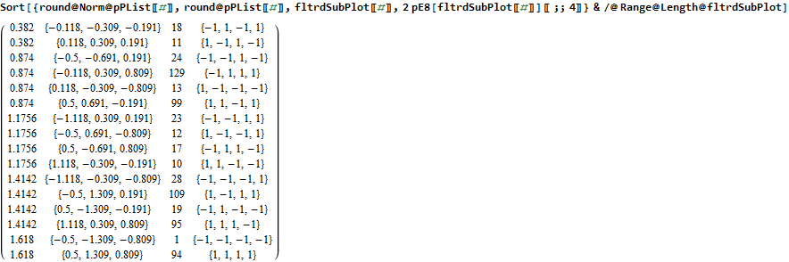
Please notice I have left in the final command of the Mathematica source code to give a hint as to the source structure of the data.