I’ve updated the .NB, .CDF and interactive demonstrations to include the ability to visualize the split octonions.
Category Archives: Physics
Klein Quartic Curves
With some Mathematica source from Leon Lampret at math.stackexchange.com, I’ve been trying to understand the link between the bitangents of octonions and the Klein Quartic Curves.
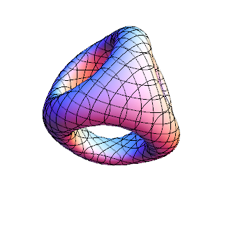
Which seems to be closely related to Greg Egan’s wonderful visualization from
http://www.gregegan.net/SCIENCE/KleinQuartic/KleinQuartic.html
The Comprehensive Split Octonions and their Fano Planes
Please see this post for updates to these graphs.
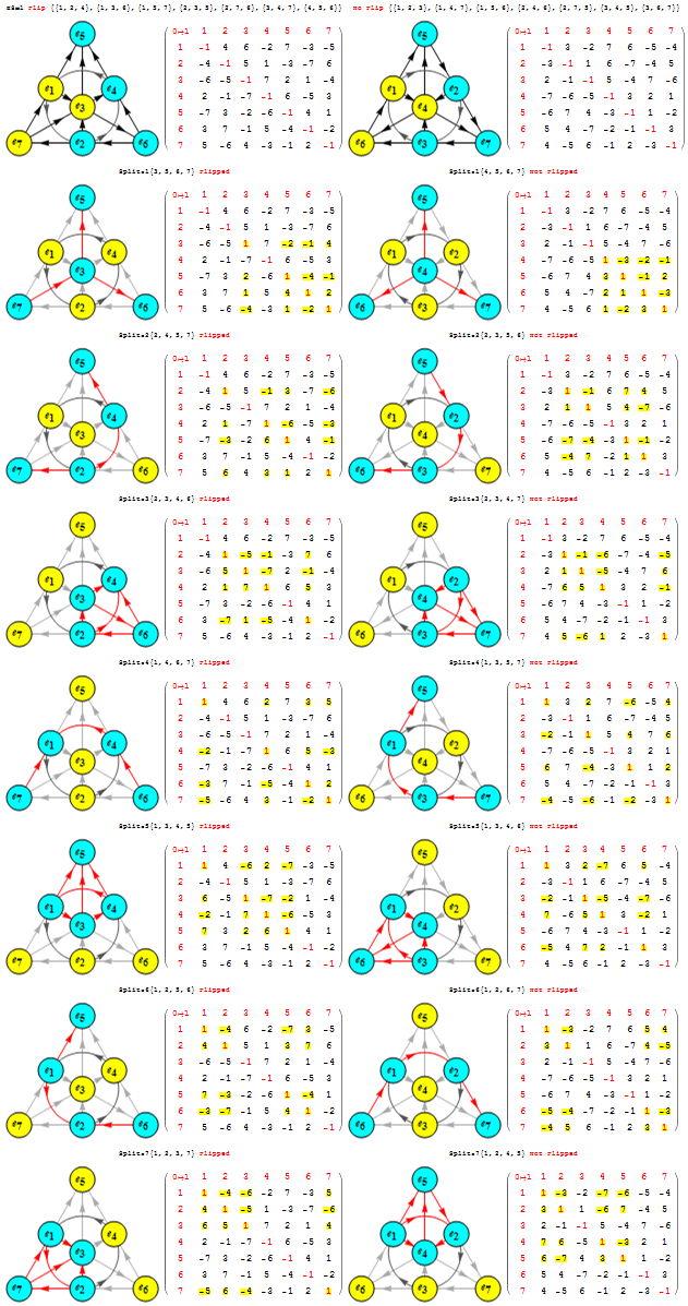
I am pleased to announce the availability of splitFano.pdf, a 321 page pdf file with the 3840=480*8 split octonion permutations (with Fano planes and multiplication tables). These are organized into “flipped” and “non-flipped” pairs associated with the 240 assigned particles to E8 vertices (sorted by Fano plane index or fPi).
There are 7 sets of split octonions for each of the 480 “parent” octonions (each of which is defined by 30 sets of 7 triads and 16 7 bit “sign masks” which reverse the direction of the triad multiplication). The 7 split octonions are identified by selecting a triad. The complement of {1,2,3,4,5,6,7} and the triad list leaves 4 elements which are the rows/colums corresponding to the negated elements in the multiplication table (highlighted with yellow background). The red arrows in the Fano Plane indicate the potential reversal due to this negation that defines the split octonions. The selected triad nodes are yellow, and the other 4 are cyan (25MB).
These allow for the simplification of Maxwell’s four equations which define electromagnetism (aka.light) into a single equation.
I believe this is the only comprehensive presentation of all 3840 Split Fano Planes with their multiplication tables available.
Below is the first page of the comprehensive split octonion list.
Detail explanation of E8 Integration with Octonions, Particles, and the Periodic Table
Please see Integrated E8, Binary, Octonion for a tutorial that explains the detail of the content of Fano.pdf. It outlines the relationships in the integration of E8 with Octonions, Binary, Particles, NKS, and the Periodic Table of Elements. Other formats are also available (.ppt or .pps and .pdf).
Created a simpler Fano plane and cubic .pdf
A simpler version of Fano.pdf is here FanoOnly.pdf (15MB).
Improved complete index of E8, Binary, Octonions, Particles, NKS CA & Periodic Table
The main change was an improved association of the 120 periodic table elements to the 120 root vectors weighted by their simple root grading. See the full 241 page reference here.

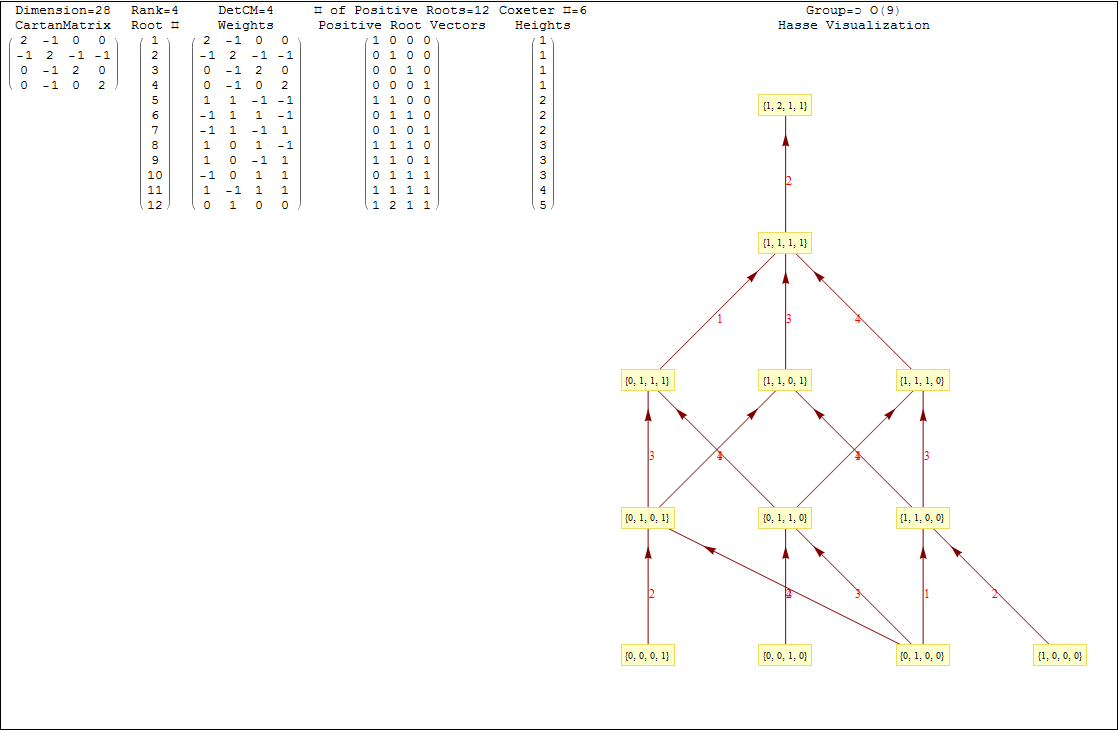
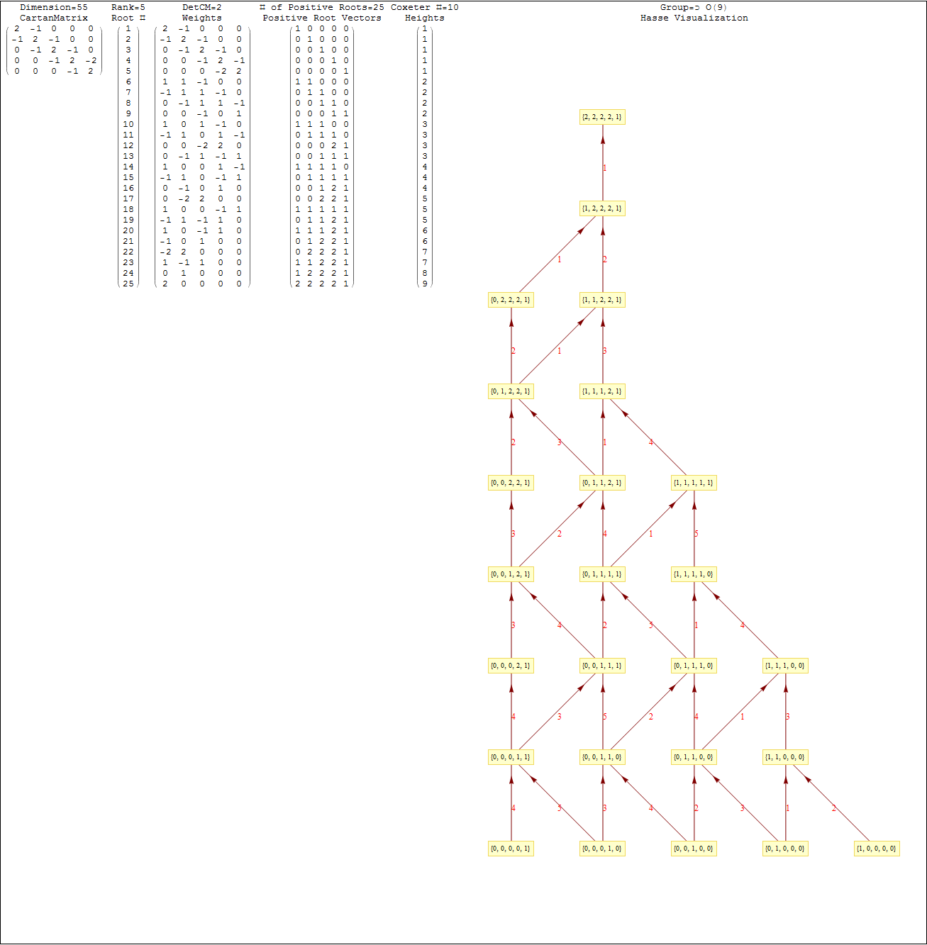
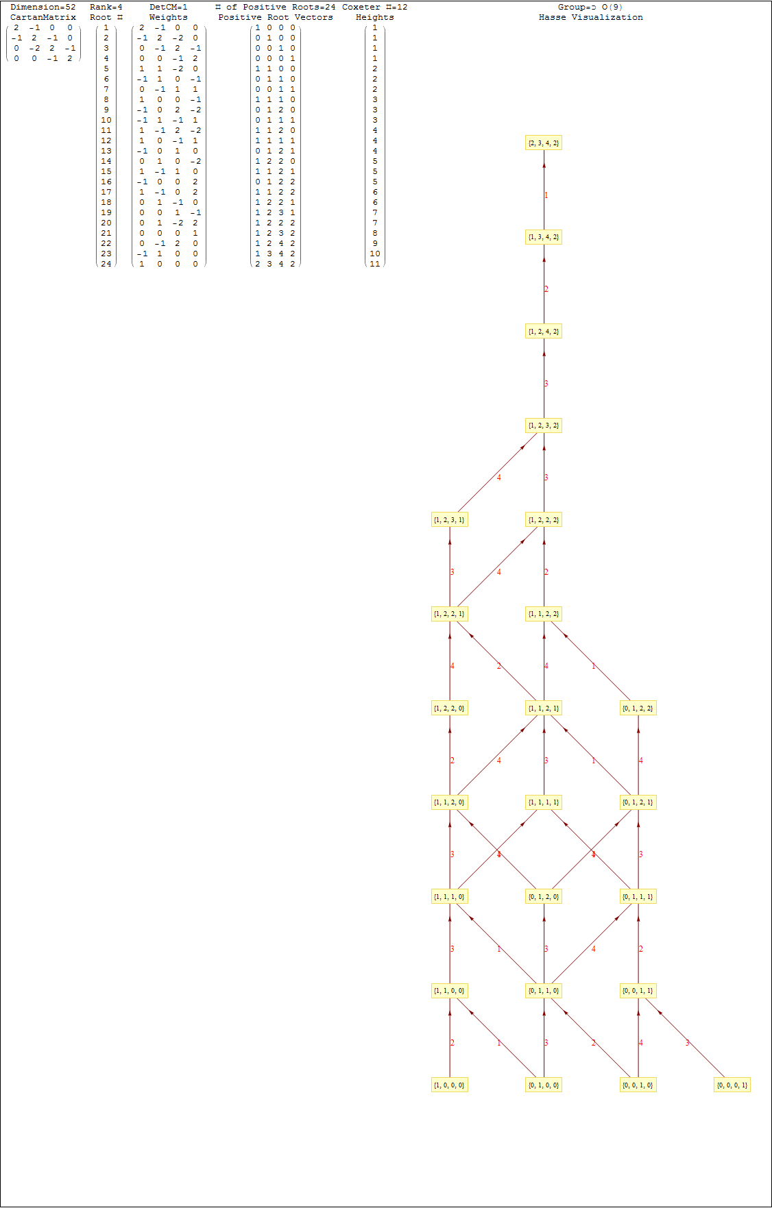
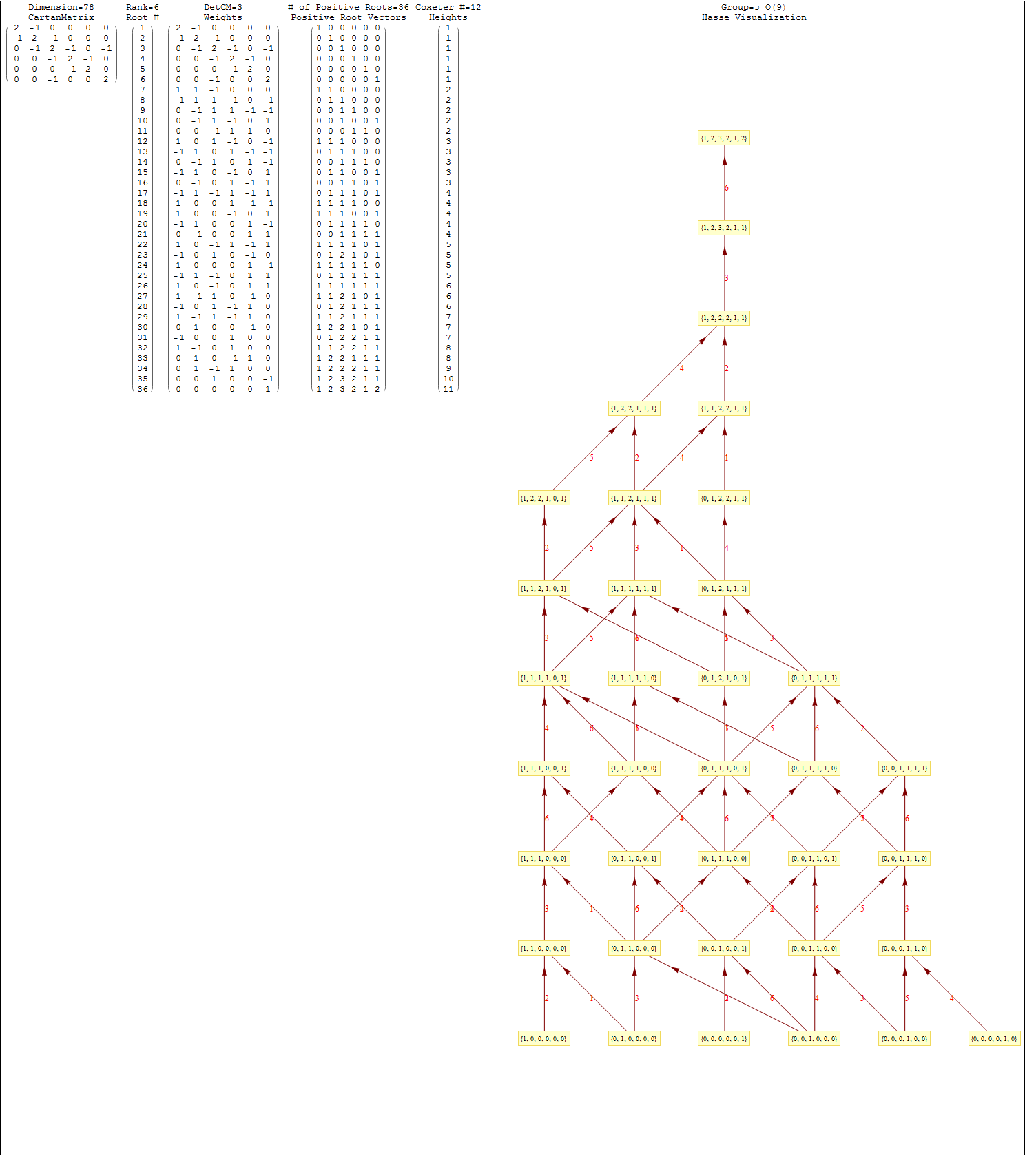
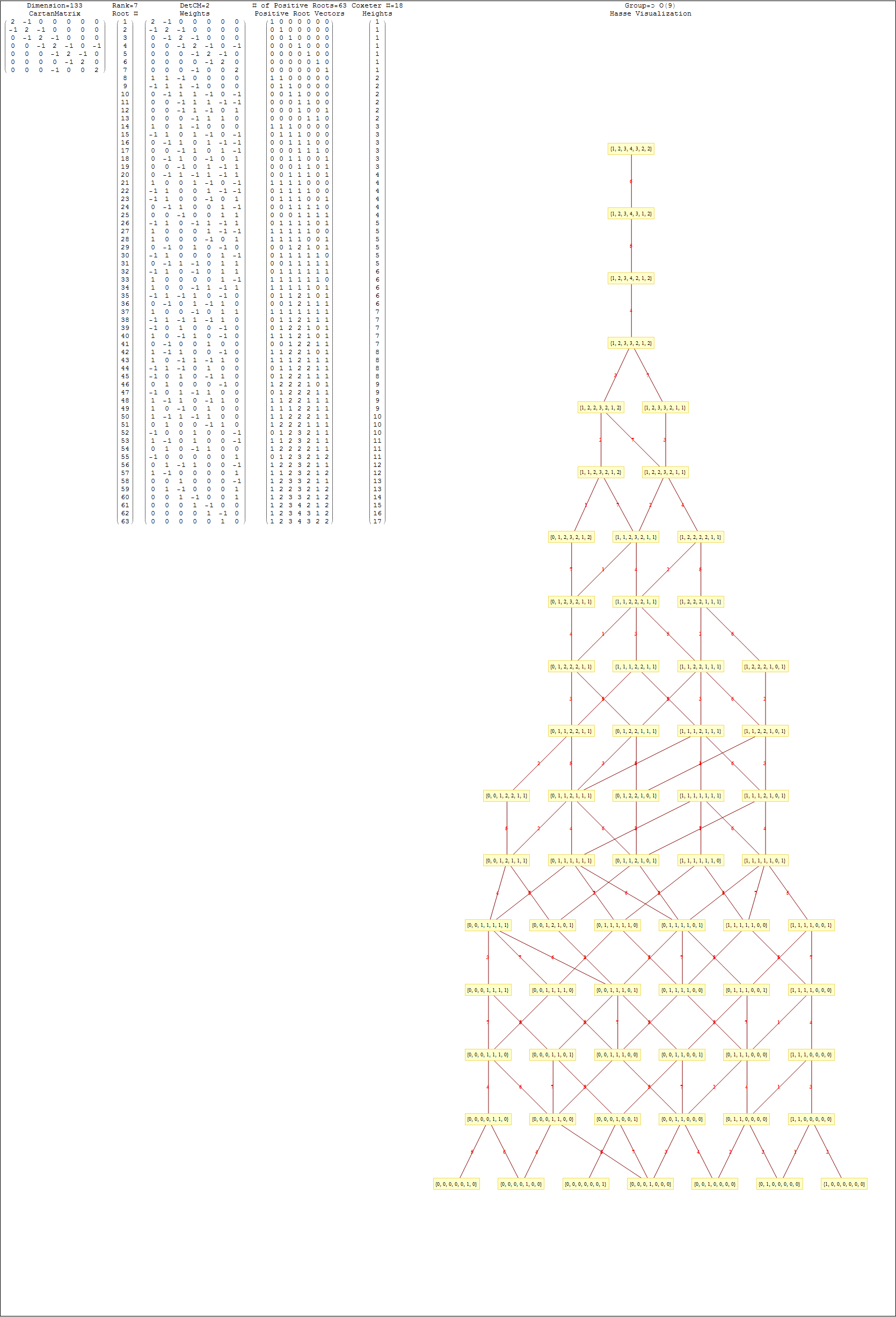
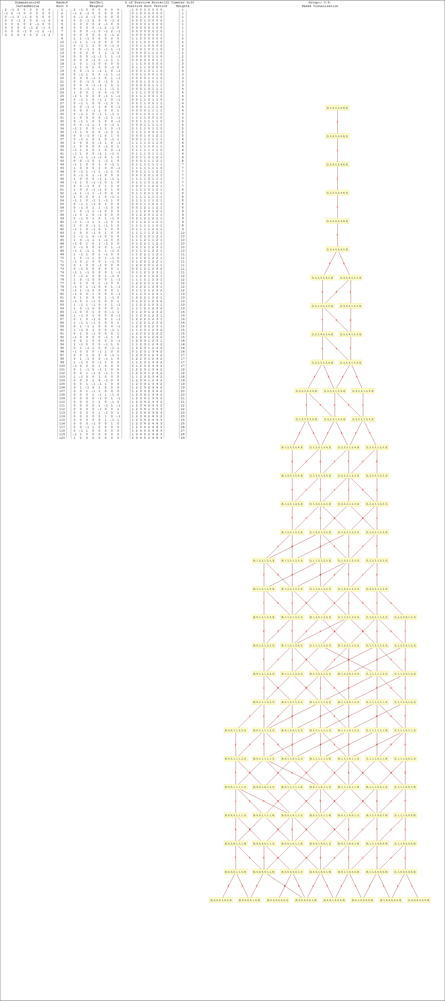
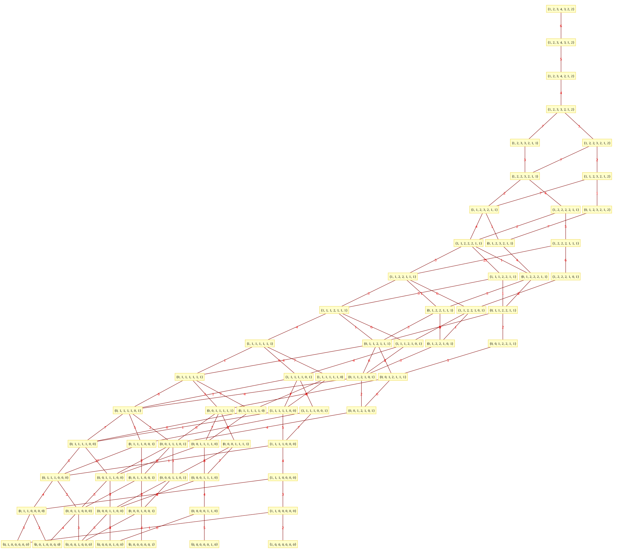
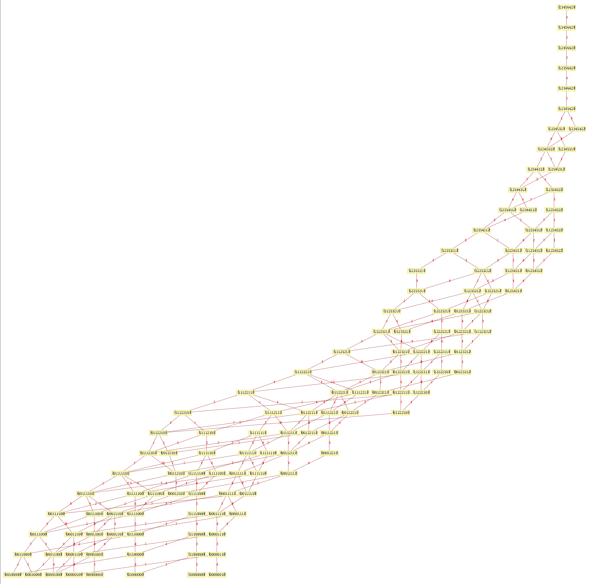
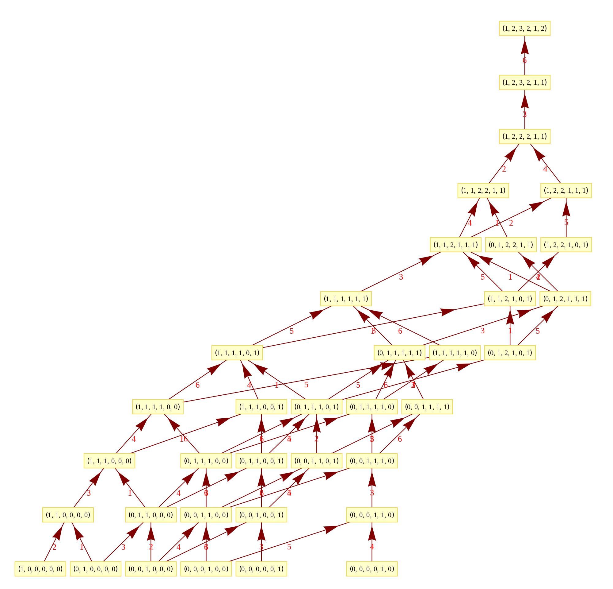
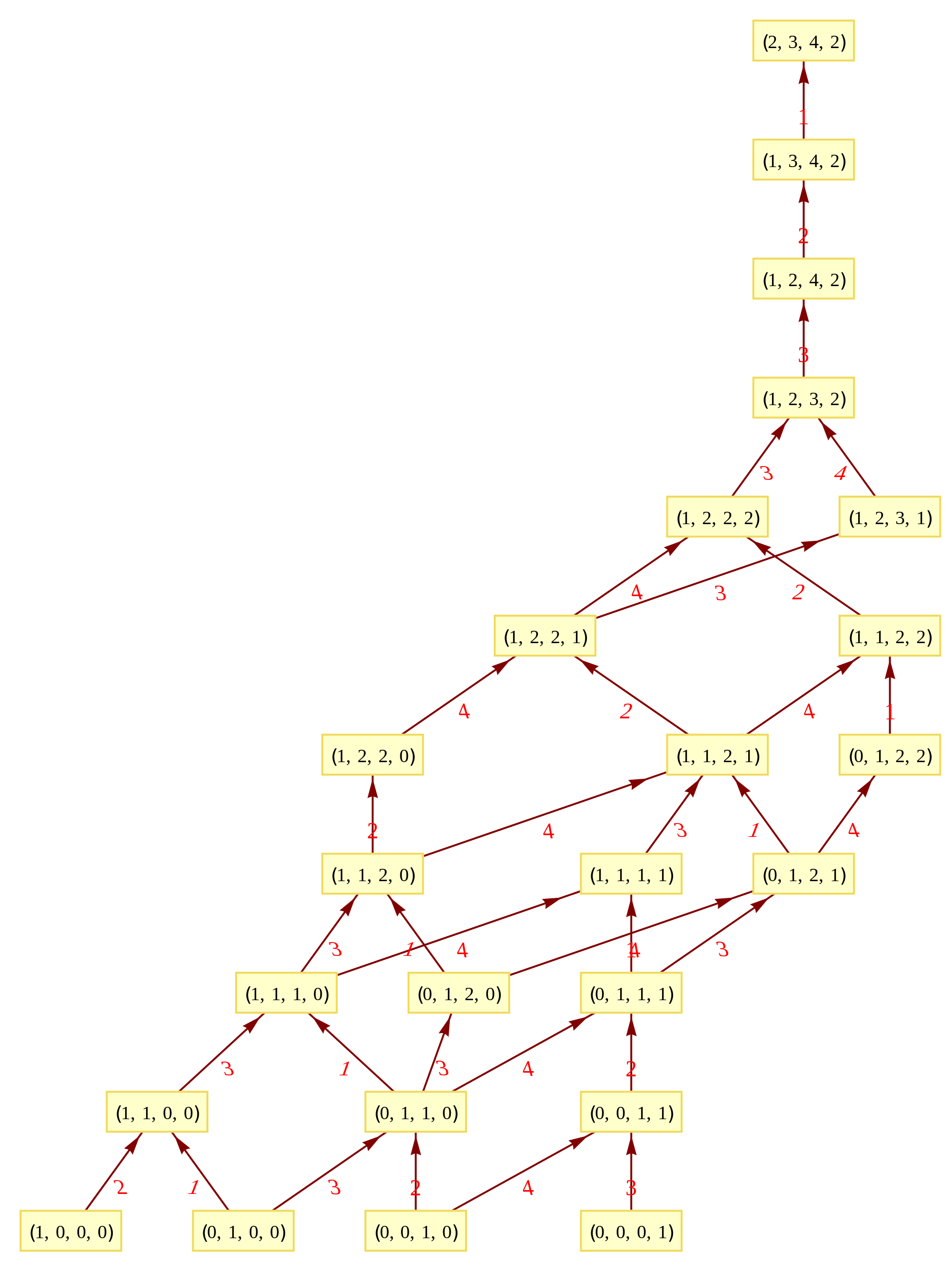
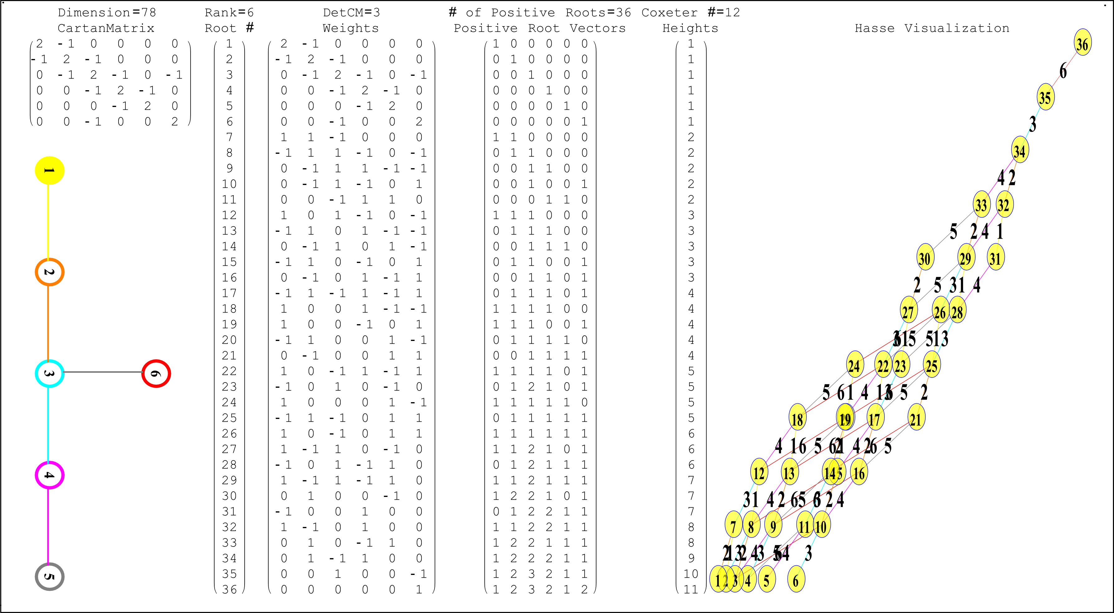
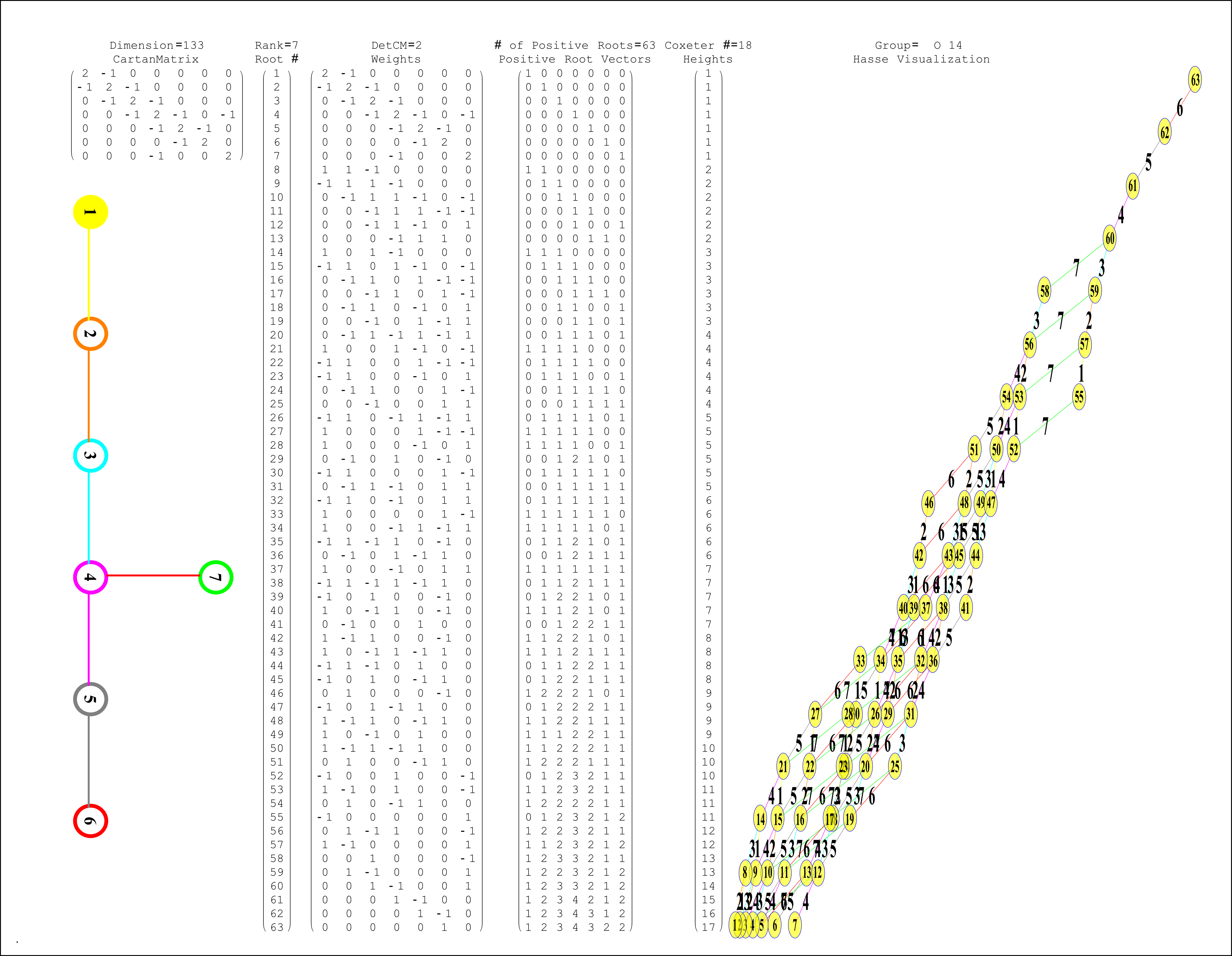
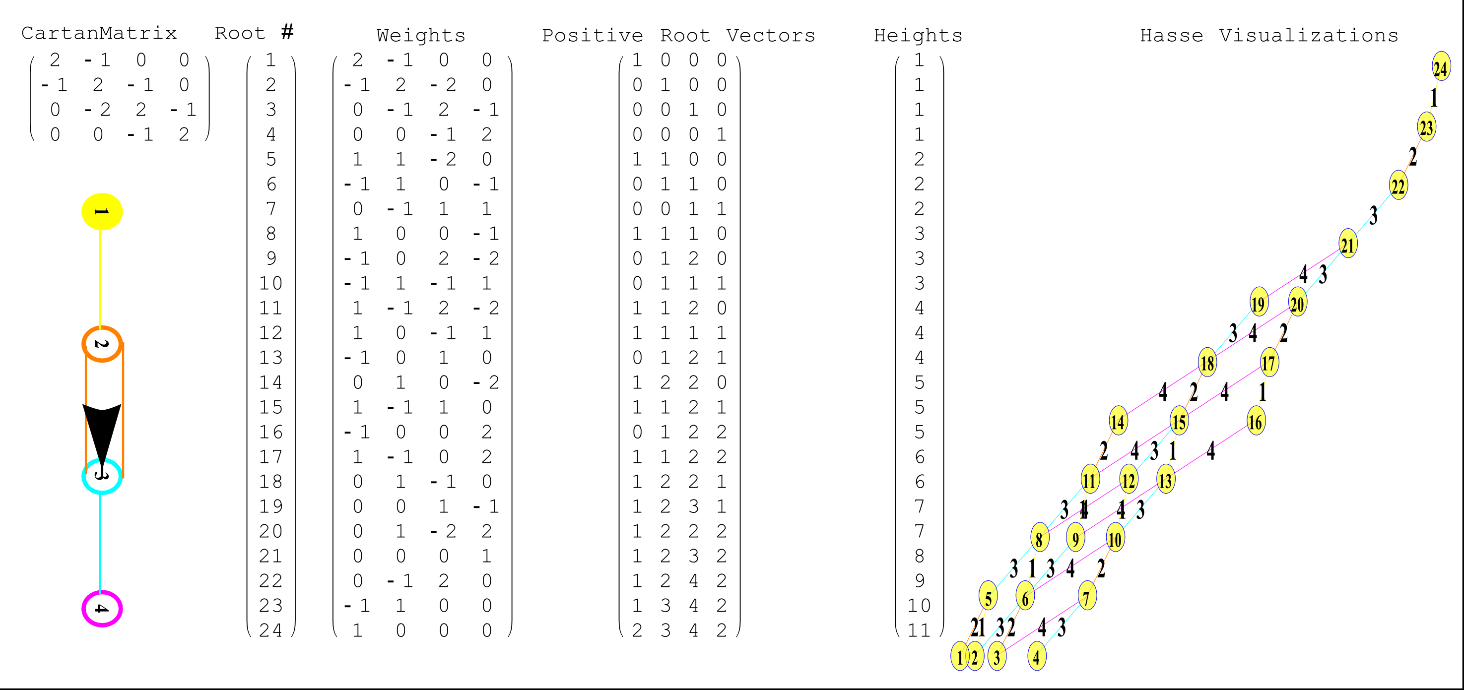
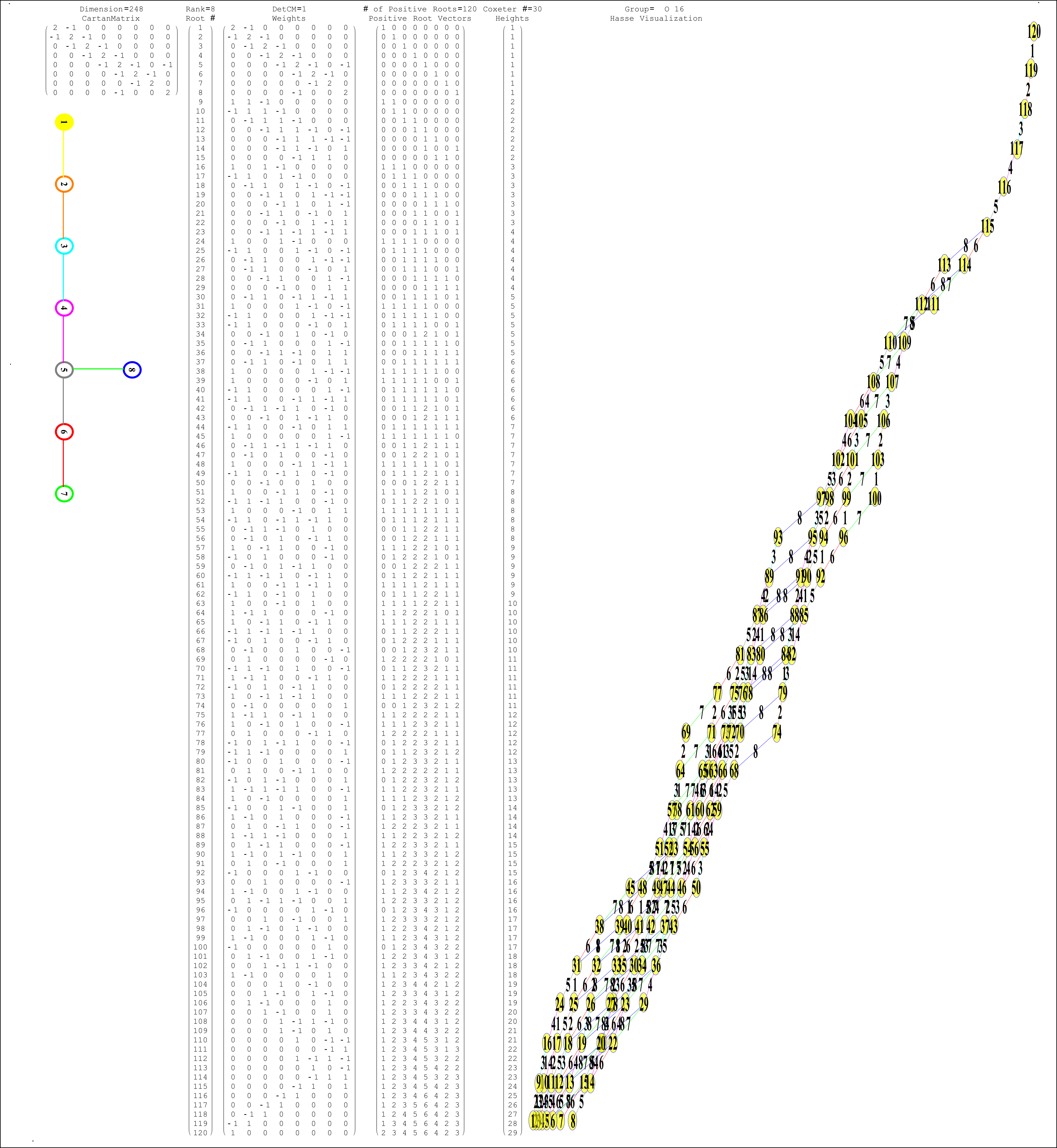
Improved the Hasse Visualizations
I’ve added better edge coloring and added edge root vector information (for the added simple root used).
Integration of the Atomic Elements to E8 and Octonions
While it still needs some work – I’ve integrated the atomic elements to the Octonions, E8 and theoretical Lisi eSM model particle assignments (along with Wolfram’s NKS Cellular Automata linked to the Clifford Algebra/Pascal Triangle binary assignments). I have combined all these visualizations with the 2D/3D electron orbitals (based on the symmetry of the {n,l,m,s} quantum numbers (from the Stowe-Janet-Scerri Periodic Table. I totally understand this is not easy to dig into w/o some effort, but … it looks cool 😉
It is shown in an updated version of Fano.pdf. This is a very large and complex 30Mb file – with 241 pages. It shows the Lisi particle assignments, the E8 roots, split real even (SRE) E8 vertex and the Lisi “physics rotation”. It also shows two Fano plane and cubic derived from the symmetries of the E8 particle assignments (and all the relevant construction of it). See the interactive demo or the Mathematica Notebook for a more “navigational look” at the integration.

Created a new 4D Stowe-Janet-Scerri Periodic Table
I’ve replaced the standard periodic table in the 7th “Chemistry Pane” of my E8 visualizer with a 2D/3D/4D Stowe-Janet-Scerri version of the Periodic Table.
Interestingly, it has 120 elements, which is the number of vertices in the 600 Cell or the positive half of the 240 E8 roots. It is integrated into VisibLie_E8 so clicking on an element adds that particular atomic number’s E8 group vertex number to the 3rd E8 visualizer pane.
The code is a revision and extension of Enrique Zeleny’s Wolfram Demonstration
A few screen shots….


2D and 3D electron orbitals for each element


MyToE updated from 2013 Planck Spacecraft and 2012 LHC results
With the recent publication of results for the Planck spacecraft results and the recent LHC Higgs results for the discovery of a 125(+/-1.5)GeV Higgs boson, I thought I would publish the minor tweaks to my PDF ToE summary or see the Mathematica notebook here. Enjoy!
It is interesting to note that my original paper from ’98 (updated ’01) Constants-A_New_Look.pdf contains this new Planck CMB probe result for a Hubble constant of H0=67.133 km/s/Mpc, which is at odds with WMAP, COBE, and prior estimates.
This old paper has a Higgs mH=98.137 GeV, which is around the minima of the ChiSquared value for Higgs. This was quickly excluded by FermiLab results around that time. The basic Higgs prediction relies purely on the dimensionality of the model and the Planck constant. Adding a factor of 2^1/2 gave an aesthetically pleasing mH=147.98 in a ’07 paper here. This was close to a June ’11 FermiLab CDF bump at 148 GeV. Unfortunately D0 at FermiLab didn’t confirm it.
Interestingly between the ’01 and the ’07 papers, one of the Higgs mass models I used 2^1/4 (not 2^1/2) and puts mH=124.43 GeV – right where LHC ATLAS and CMS seem to have found it. This same model also (fairly) accurately integrates this to the Fermi Constant and vacuum expecation (VEV).
The bottom line, my model describes results that are within the most current and accurate experimentally measured data, including the LHC Higgs and Planck CMB probes.
ToE Summary

It is interesting to note that the added factor of λcnv over H0, which is based on the Compton wavelength of the electron/proton mass ratio (as is gc), precisely accommodates the Hubble tension!