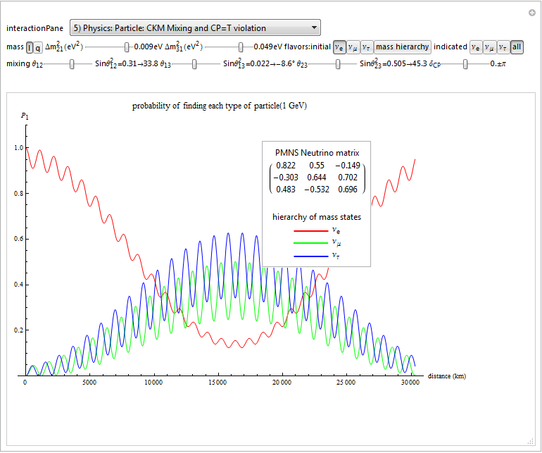
I’ve improved on a great Wolfram demonstration from Balázs Meszéna on Neutrino Oscillations by adding capabilities to view both the PMNS and CKM unitary triangle matrices, print and reference my ToE Neutrino mass predictions, which now accomodate the Koide relationships in particle masses.
Check out the new demonstrations using free interactive web plugin , .CDF, or .NB (for licensed Mathematica users) and social media integrations for comments, pages and posts.
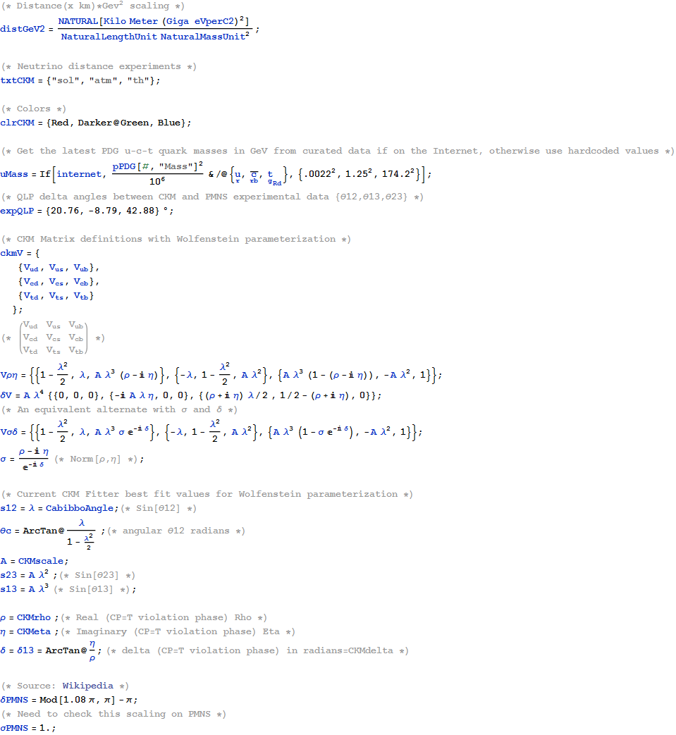
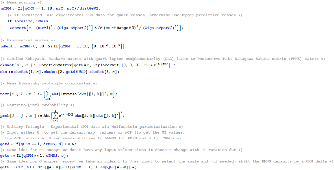
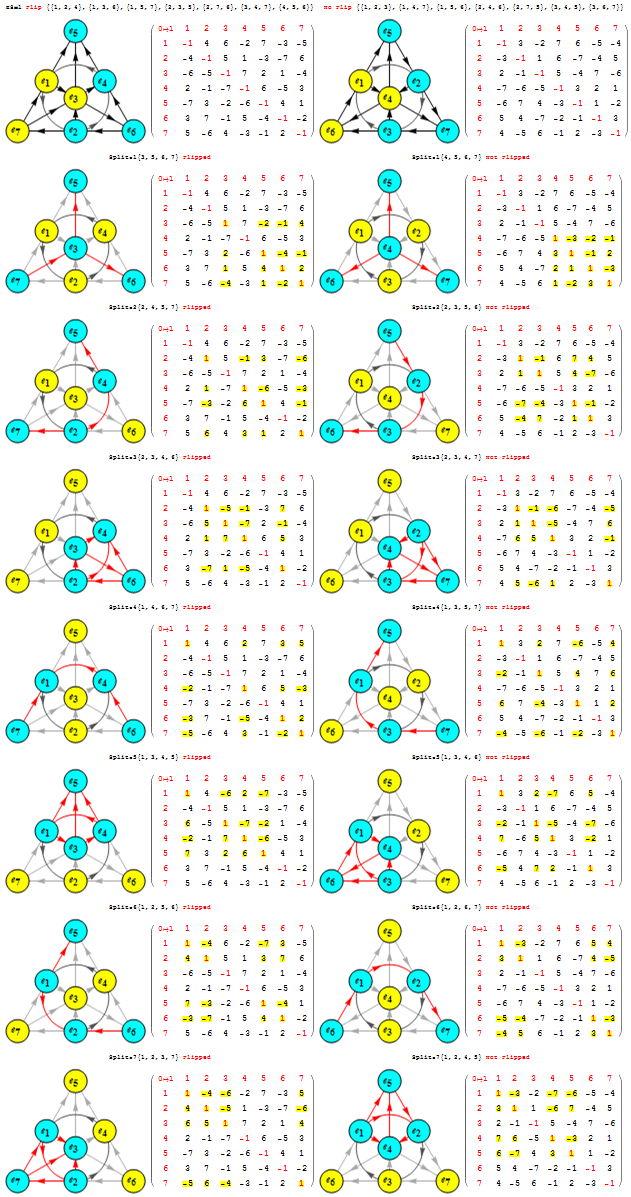
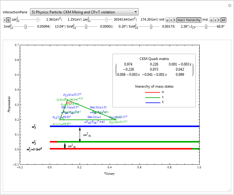
This new pane (#5) presents the Unitarity of CP=T violations by combining the Lepton (Neutrino) Pontecorvo-Maki-Nakagawa-Sakata matrix (PMNS) with the Quark Cabibbo-Kobayashi-Maskawa (CKM) mixing matrix calculations through the Quark-Lepton Complementarity (QLC).
I am also working to incorporate the Koide particle mass relations to MyToE predictions.
Code snippets showing the CKM and PMNS matrix calculations based on the UI.