All posts by jgmoxness
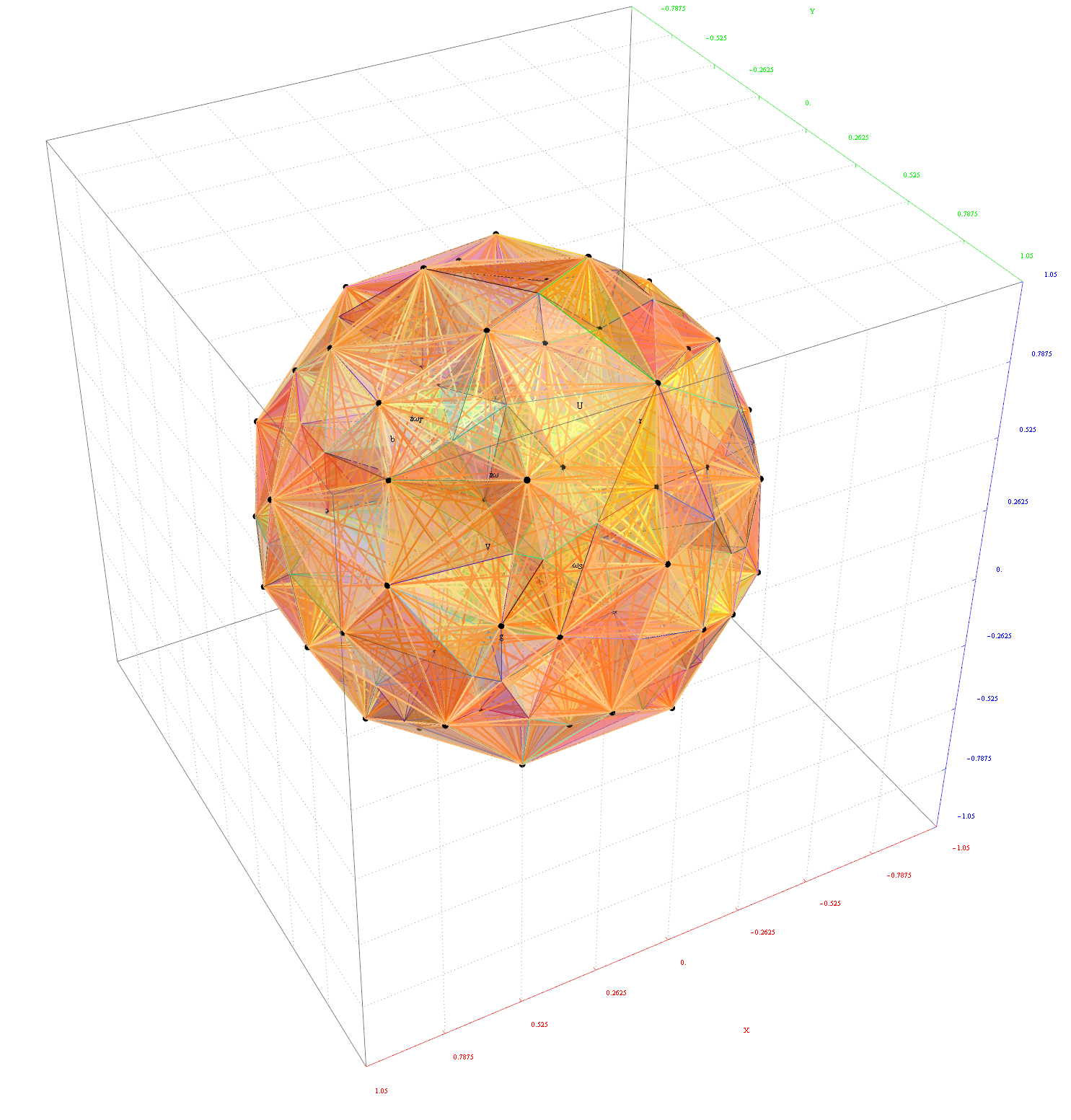
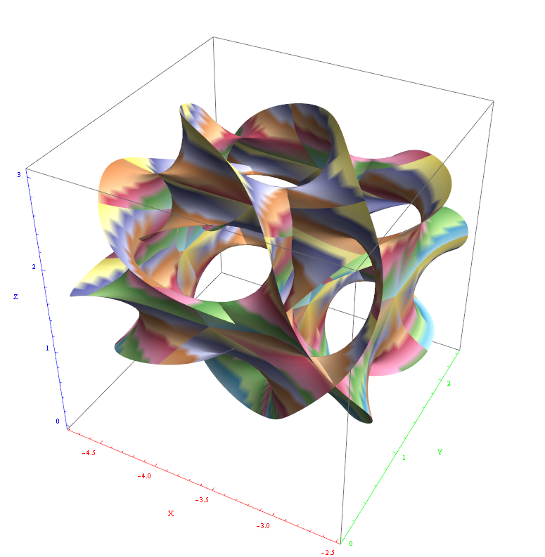
E8 to H4 Folding Amplituhedron Surface Visualization
…nuff said, enjoy!
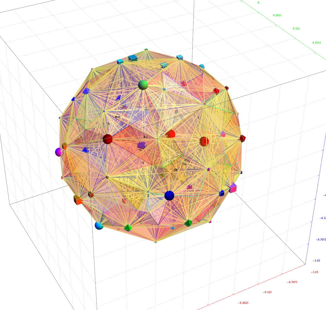
or in “physics mode”
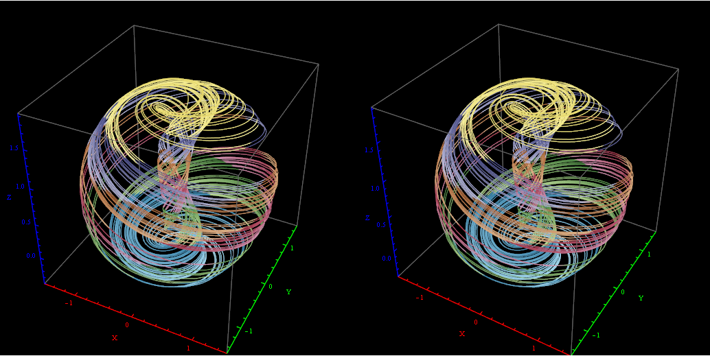
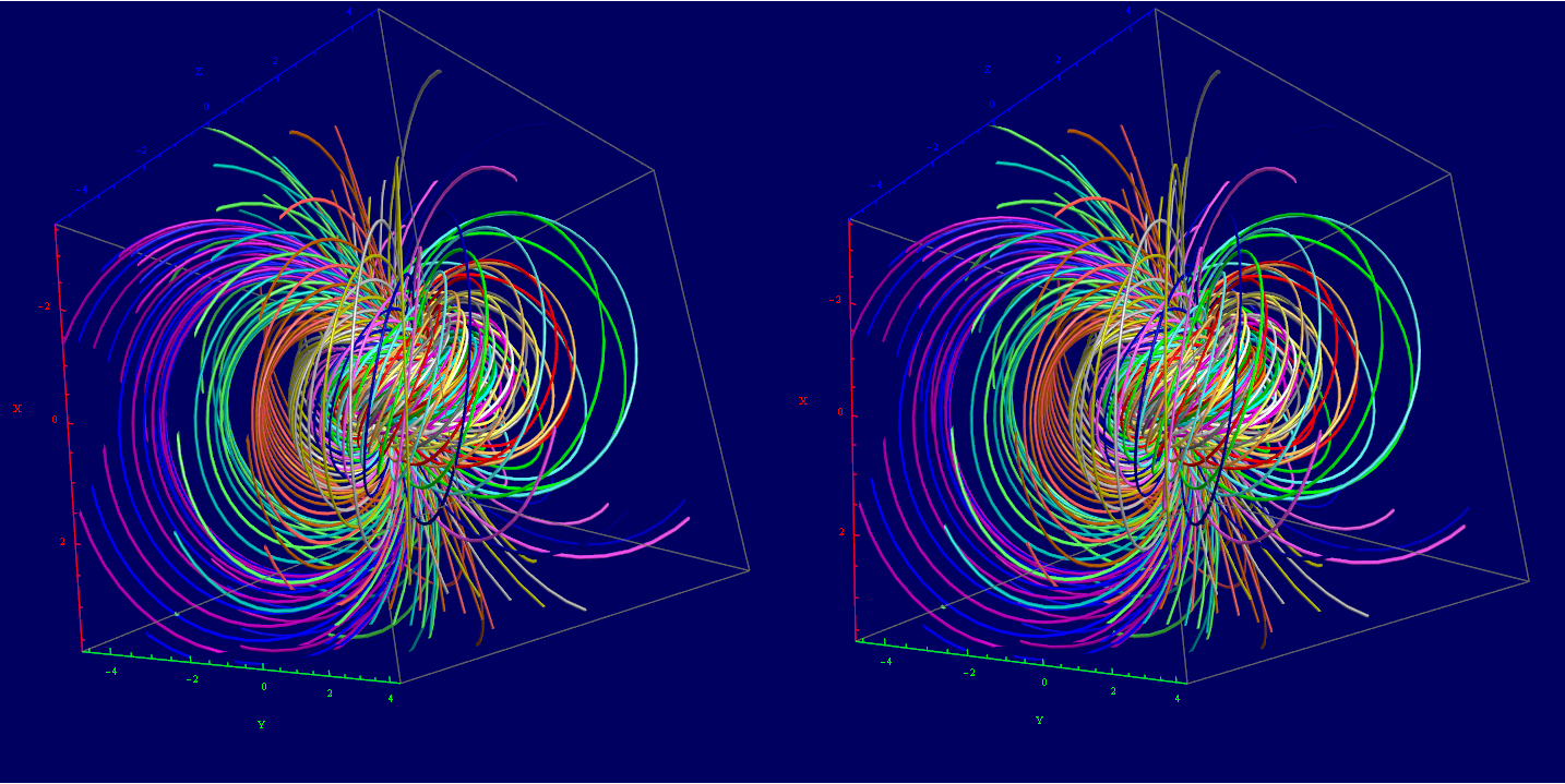
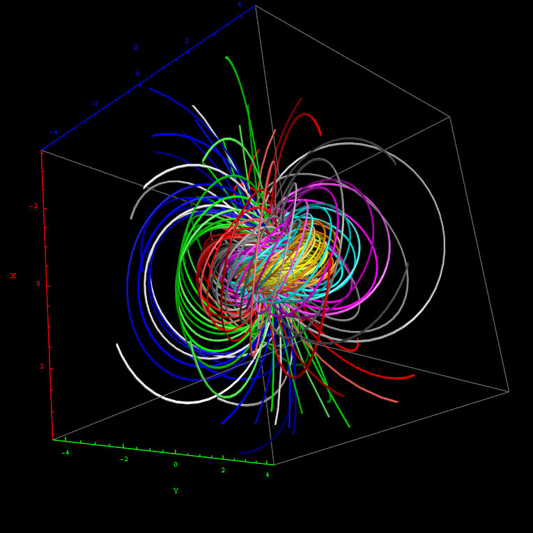
Hopf Fibration and Chaotic Attractors, etc.
I’ve added some new features to my VisibLie_E8 ToE Demonstration. Some of it comes from Richard Hennigan’s Rotating The Hopf Fibration and Enrique Zeleny’s A Collection Of Chaotic Attractors . These are excellent demonstrations that I’ve now included with the features of my integrated ToE demonstration, since they are not only great visualizations, but relate to the high-dimensional physics of E8, octonions and their projections. This gives the opportunity to change the background and color schemes, as well as output 3D models or stereoscopic L/R and red-cyan anaglyph images.
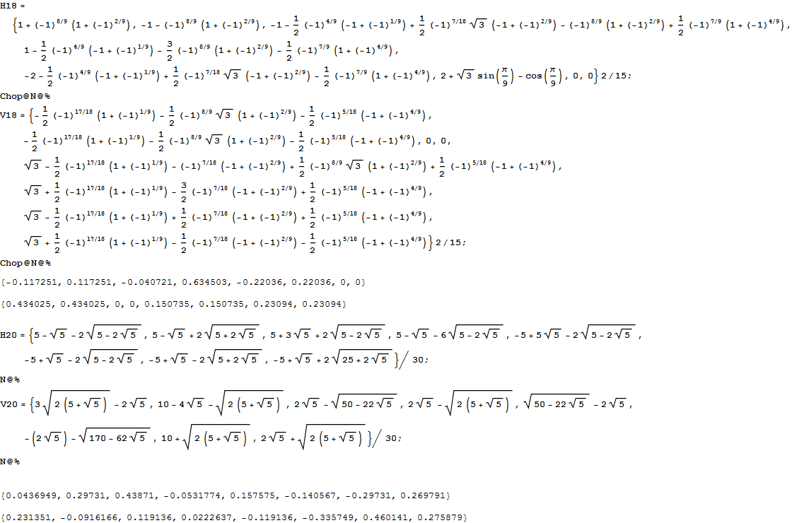
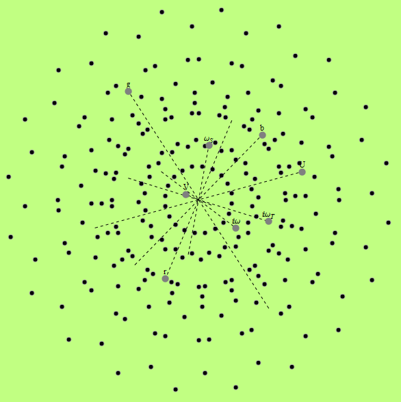
I’ve also used David Madore’s help to calculate the symbolic value of the E7 18-gon and 20-gon symmetries of E8. It uses the nth roots of unity (18 and 20, in this case) and applies a recursive dot product matrix based on the Weyl group centralizer elements of a given conjugacy class of E8. I ended up using a combination of Mathematica Group Theory built-in functions, SuperLie and also LieART packages. These symbolic projection values are:
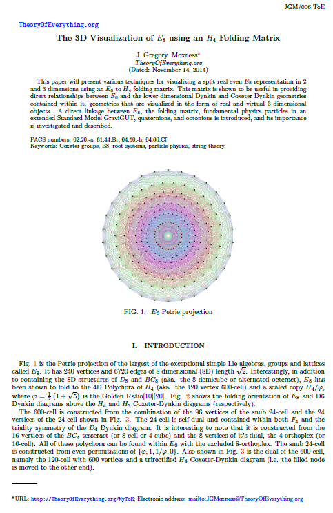
My latest paper on E8, the H4 folding matrix, and integration with octonions and GraviGUT physics models.
The full paper with appendix can be found on this site, or w/o appendix on viXra. (13 pages, 14 figures, 20Mb). The 22 page appendix contains the E8 algebra roots, Hasse diagram, and a complete integrated E8-particle-octonion list.
Abstract:
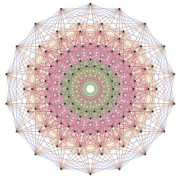
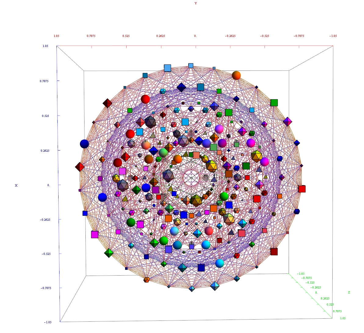
This paper will present various techniques for visualizing a split real even E8 representation in 2 and 3 dimensions using an E8 to H4 folding matrix. This matrix is shown to be useful in providing direct relationships between E8 and the lower dimensional Dynkin and Coxeter-Dynkin geometries contained within it, geometries that are visualized in the form of real and virtual 3 dimensional objects. A direct linkage between E8, the folding matrix, fundamental physics particles in an extended Standard Model GraviGUT, quaternions, and octonions is introduced, and its importance is investigated and described.
If you would like to cite this, you can use this BibTex format if you like (remove the LaTex href tag structure if you don’t use the hyperref package):
Fun with 8D rotations of E8
This is a little clip containing three different 8 dimensional rotations of E8. While it may seem like a simple rotation of an object in 3-space, if you look carefully (especially the first rotation), you can see sets of vertices moving in different directions.
The object (the 240 vertices of E8 along with 1220 of 6720 edges of 8D length Sqrt[2]) is not “moving”. It is the camera that is moving in an 8 dimensional space.
Best when viewed in HD!
The previous 3D animations here and here are created by projecting the 8 dimensional object of E8 into 3 and simply rotating (spinning) that object around in 3-space. I like to call those animations 4D, since animation visualizes changes over time – a 4D space-time object if you will…
Math only version of E8 to H4 projection
E8 to 3D projection using my H4 folding matrix
Best viewed in HD mode…
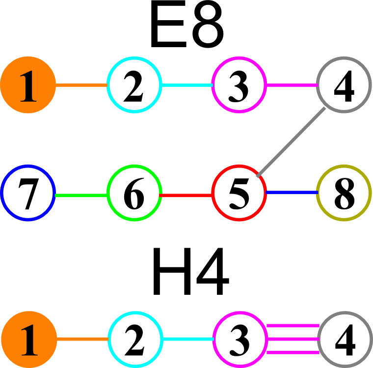
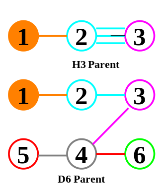
Last year I showed that the Dynkin diagram of the Lie Algebra, Group and Lattice of E8 is related to the Coxeter-Dynkin of the 600 Cell of H4 through a folding of their diagrams:
I had found the E8 to H4 folding matrix several years ago after reading several papers by Koca and another paper by Dechant, on the topic. The matrix I found is:
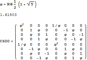
Notice that C600=Transpose[C600] and the Quaternion–Octonion like structure (ala. Cayley-Dickson) within the folding matrix. Only the first 4 rows are needed for folding, but I use the 8×8 matrix to rotate 8D vectors easily.
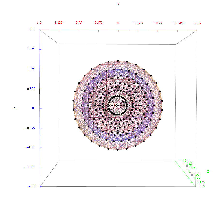
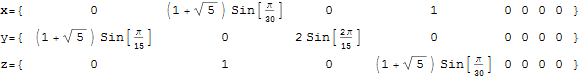
The following x,y,z vectors project E8 to its Petrie projection on one face (or 2 of 6 cubic faces, which are the same).

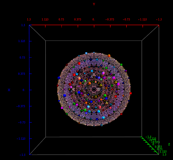
On another face are the orthonormal H4 600 cell and the concentric H4/Phi. There are 6720 edges with 8D Norm’d length of Sqrt[2], but I only show 1220 in order to prevent obscuring the nodes.
These values were calculated using the dot product of the Inverse[4*C600] with the following H4 Petrie projection vertices (aka. the Van Oss projection), where I’ve added the z vector for the proper 3D projection. Notice I am still using 8D basis vectors with the last 4 zero, as this maintains scaling due to the left-right symmetries in C600).
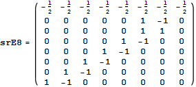
The Split Real Even (SRE) E8 vertices are generated from the root system for the E8 Dynkin diagram and its resulting Cartan matrix:
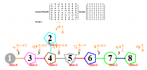
This is input from my Mathematica “VisibLie” application. It is shown with the assigned physics particles that make up the simple roots matrix entries:
 .
.
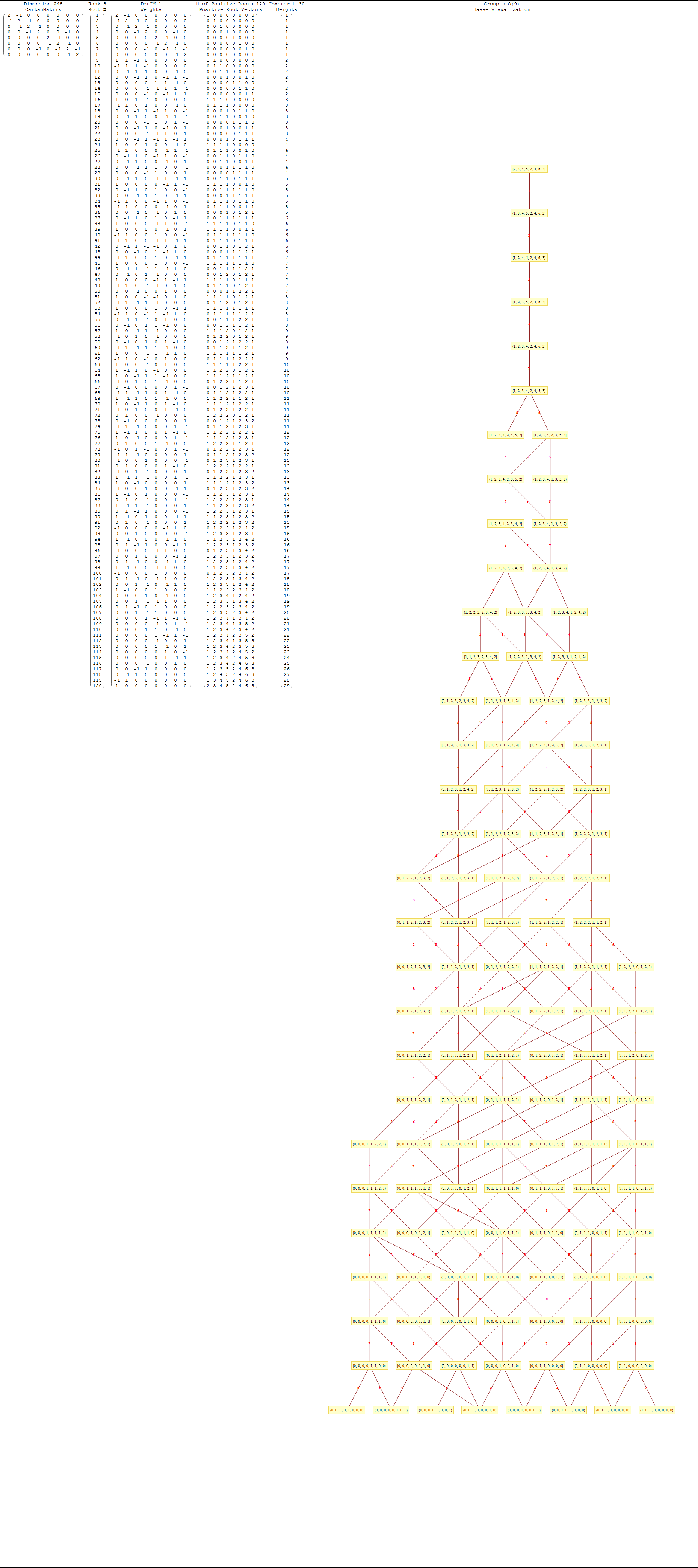
Please note, the Cartan matrix can also be generated by srE8.Transpose[srE8]
It takes Transpose[srE8] and applies the dot product against the 120 positive and 120 negative algebra roots generated by the Mathematica “SuperLie” package (shown along with its Hasse diagram, which I generate in the full version of my Mathematica notebook):
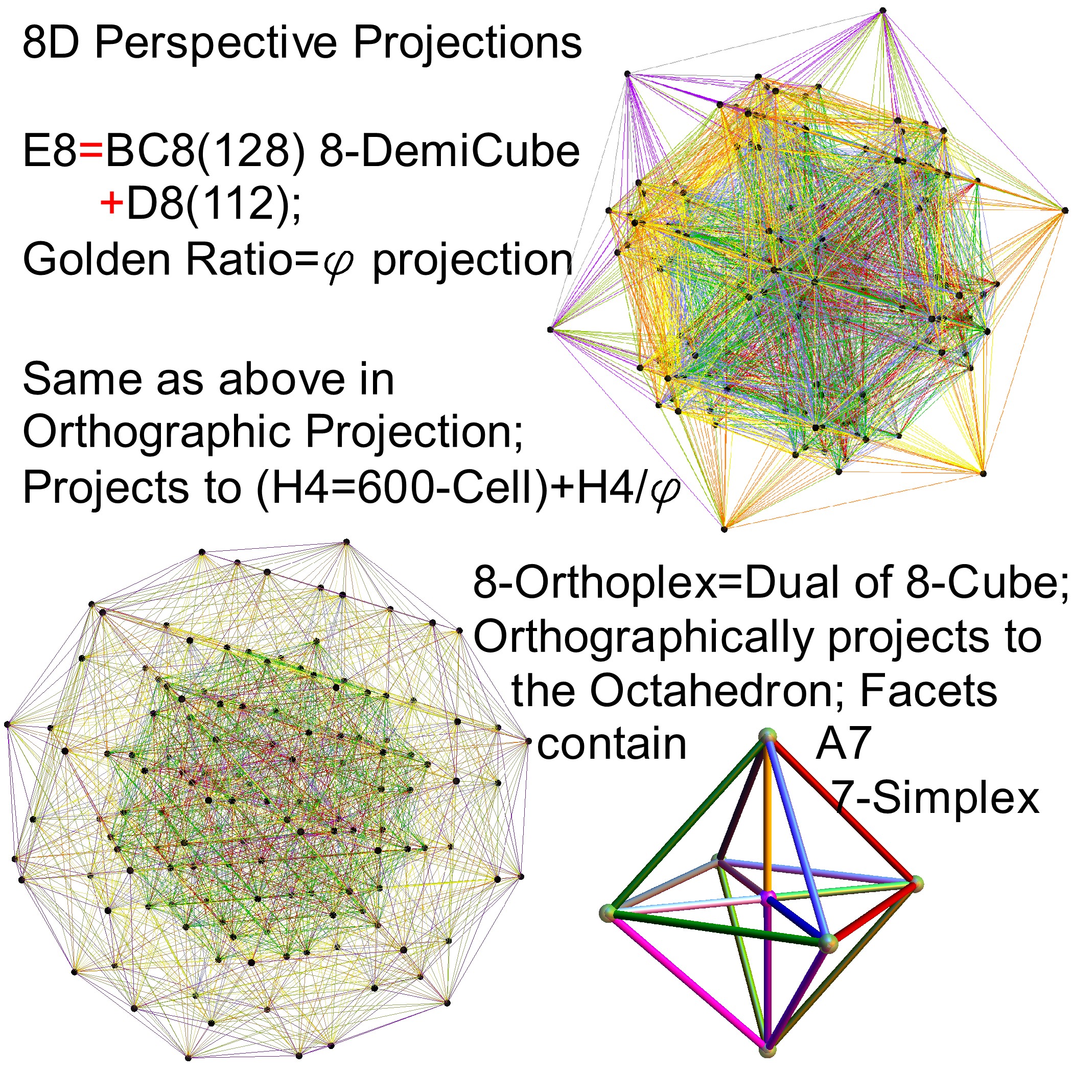
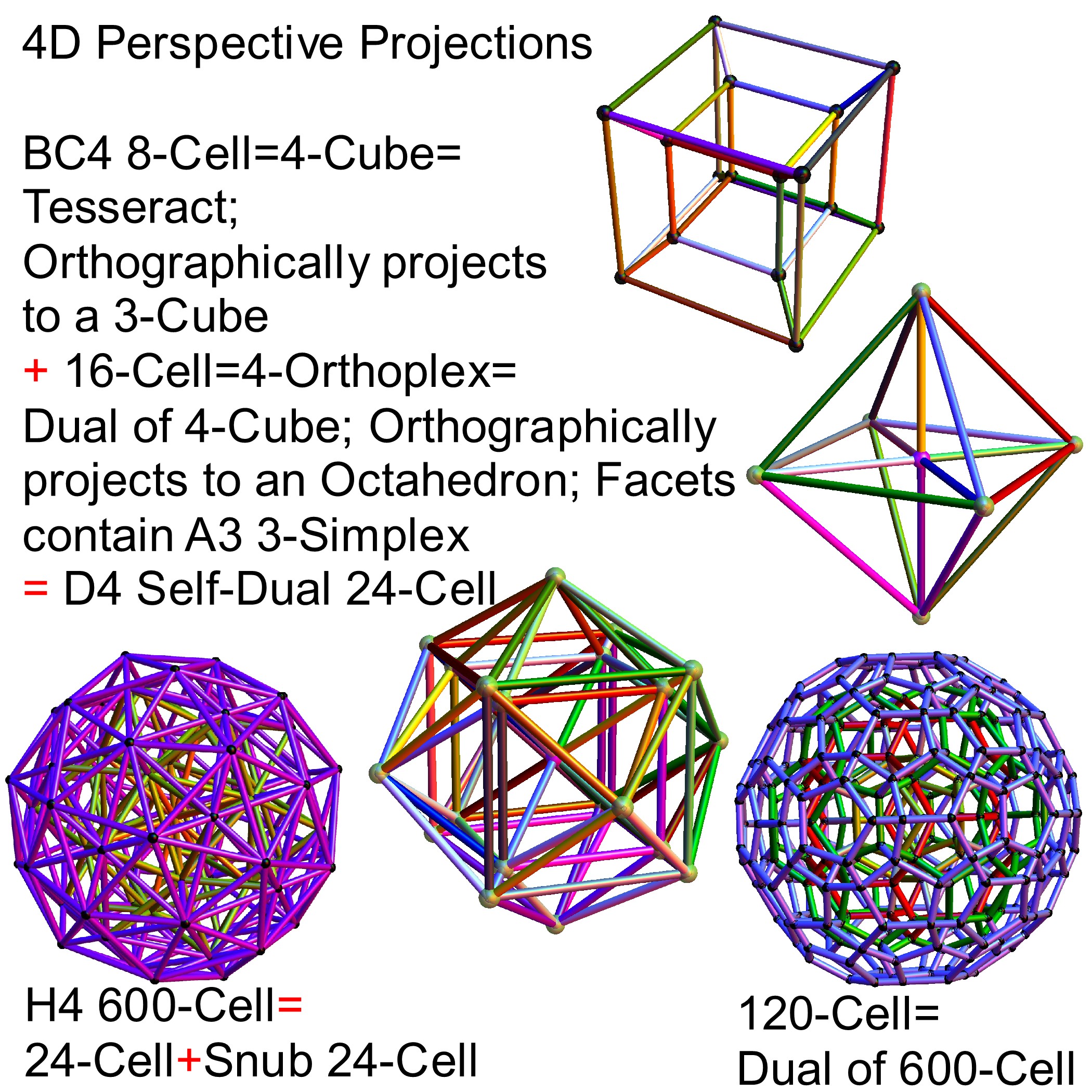
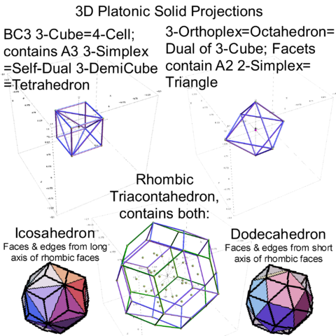
Interestingly, E8 in addition to containing the 8D structures D8 and BC8 and the 4D Polychora, contains the 7D E7, as well as the 6D structures of the Hexeract or 6 Cube. I also showed several years ago that this projects down to the 3D as the Rhombic Triacontahedron. The Rhombic Triacontahedron (of Quasicrystal fame) contains the Platonic Solids including the Icosahedron and Dodecahedron! This is shown to be done through folding of the 6-Cube using rows 2 through 4 of the E8 to H4 folding matrix!!
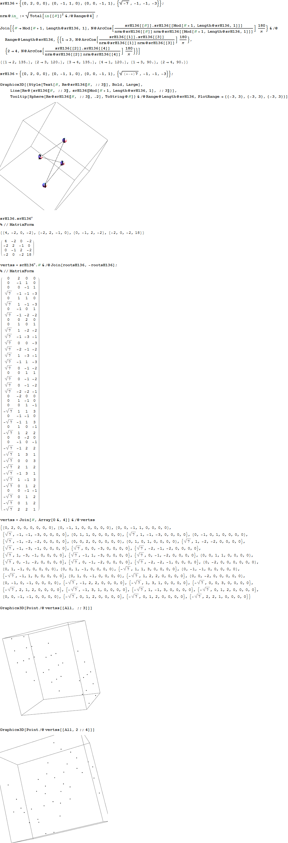
Hyperbolic Dynkin #136 Detail
In followup to John Baez’ G+ thread on Hyperbolic Dynkin diagrams, specifically on the only rank 4 compact symmetrizable diagram 136, I used my “VisibLie” notebook (which includes the “SuperLie” package for analyzing Lie Algebras) to get the following information:
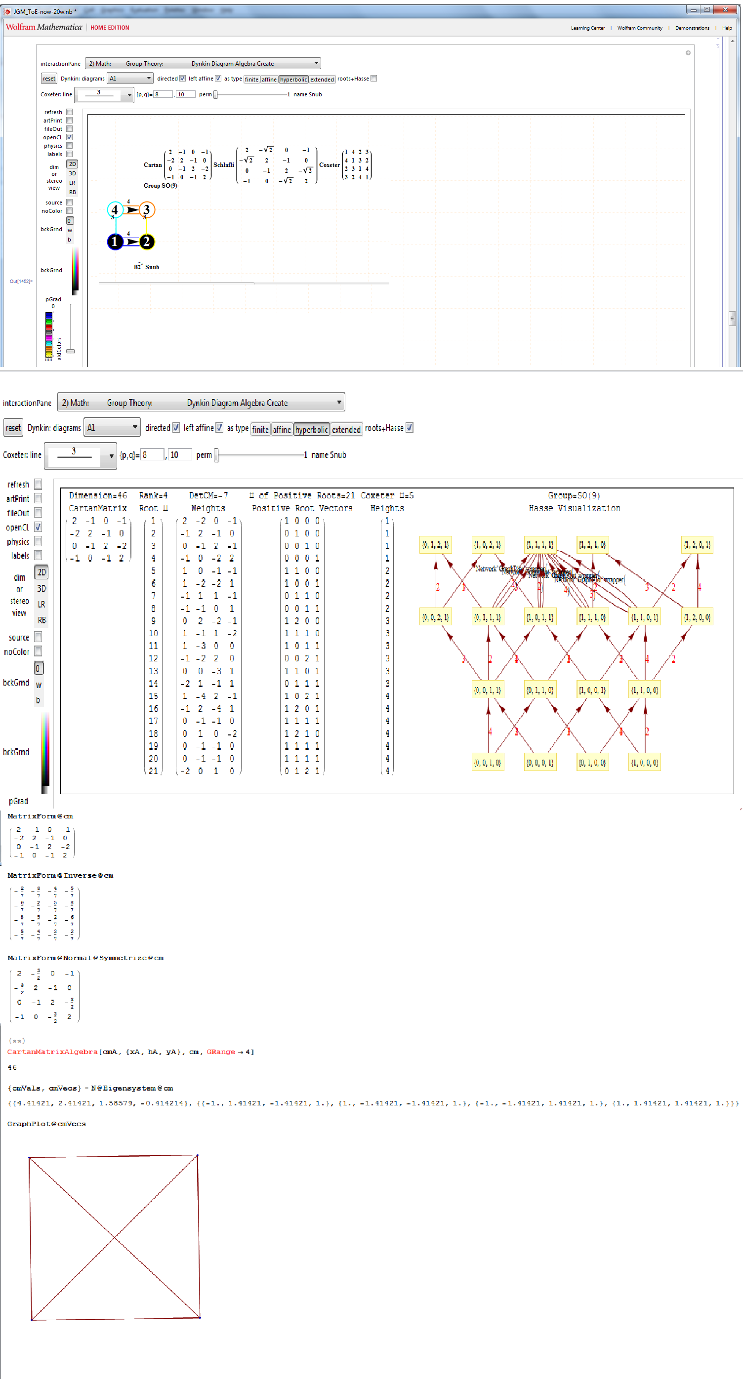
Using the “SimpLie” Google Code OpenSource software, we get Hasse diagram of:
Symmetrized Cartan matrix:
1 -1 0 -1/2
-1 2 -1 0
0 -1 2 -1
-1/2 0 -1 1
One possible set of basis vectors for this is:
srH136={{0,2,0,0},{0,-1,1,0},{0,0,-1,1},{Sqrt[-7],-1,-1,-3}};
with 4D angles between each node of:
{{1->2,135.},{2->3,120.},{3->4,135.},{4->1,120.},{1->3,90.},{2->4,90.}}
Norm’d Length between nodes is:
{2, Sqrt[2], Sqrt[2], 2}
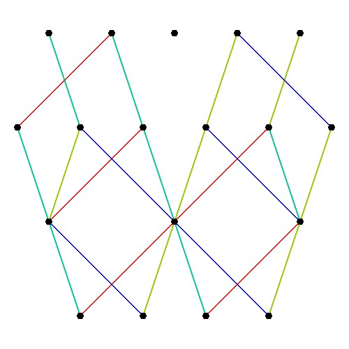
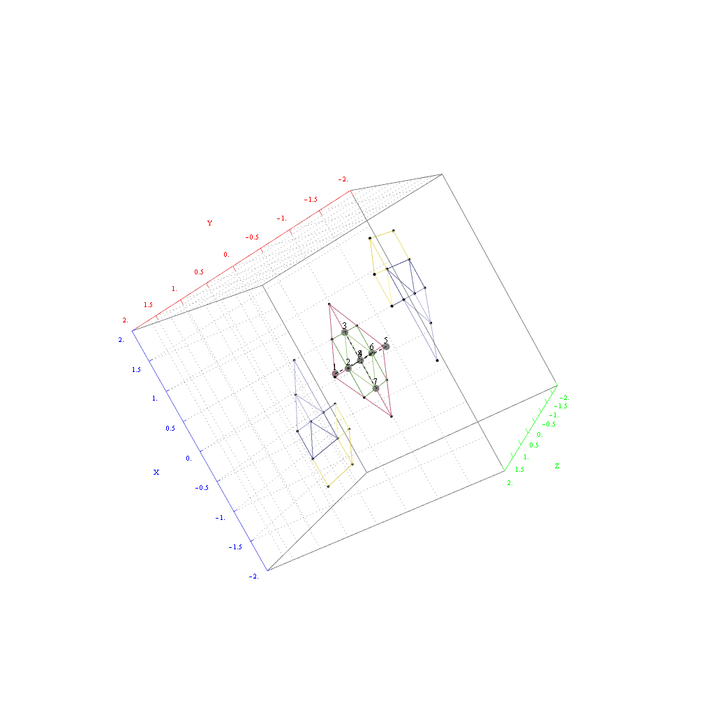
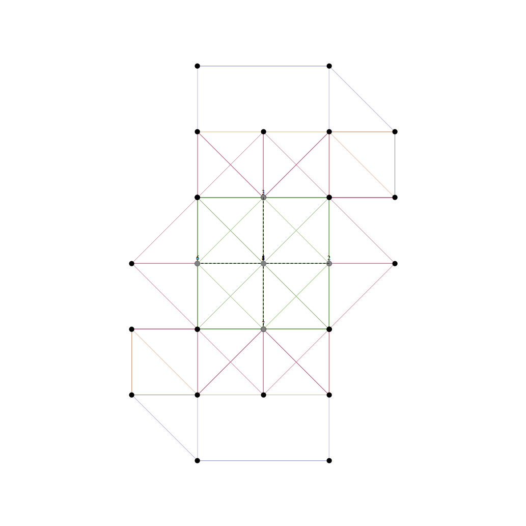
as visualized in 2D and 3D, with 42 vertices and 26 edges of Norm’d 4D length of 2 and 94 at Sqrt[2]:
Animated movies of comet Siding Spring passing Mars
Check out a little animation I did using my research tool. It is of the comet Siding Spring that gave Mars a close shave this weekend….
If you want to create a version yourself, all you need is the free Wolfram CDF player and go to my interactive visualization tool at:
http://theoryofeverything.org/theToE/visualizations/interactive/
Select the NBody Gravitational Universe simulation and select the “Recombination” epoch (the last one on the timeline).
Please note, there are two distance scales (outer planets to start, and quickly switches to inner planets as it gets close to Mars).
The planets are scaled relative to each other in each of these scales, but not relative to the Astronomical Unit distance scale between them.
BTW – The Sun is not shown, since at that planetary scale it is actually bigger than the frame of the animation 🙂
The time scale goes from last year to next year. It changes from linear around this weekend (0s) and goes exponential on the outer orbits.
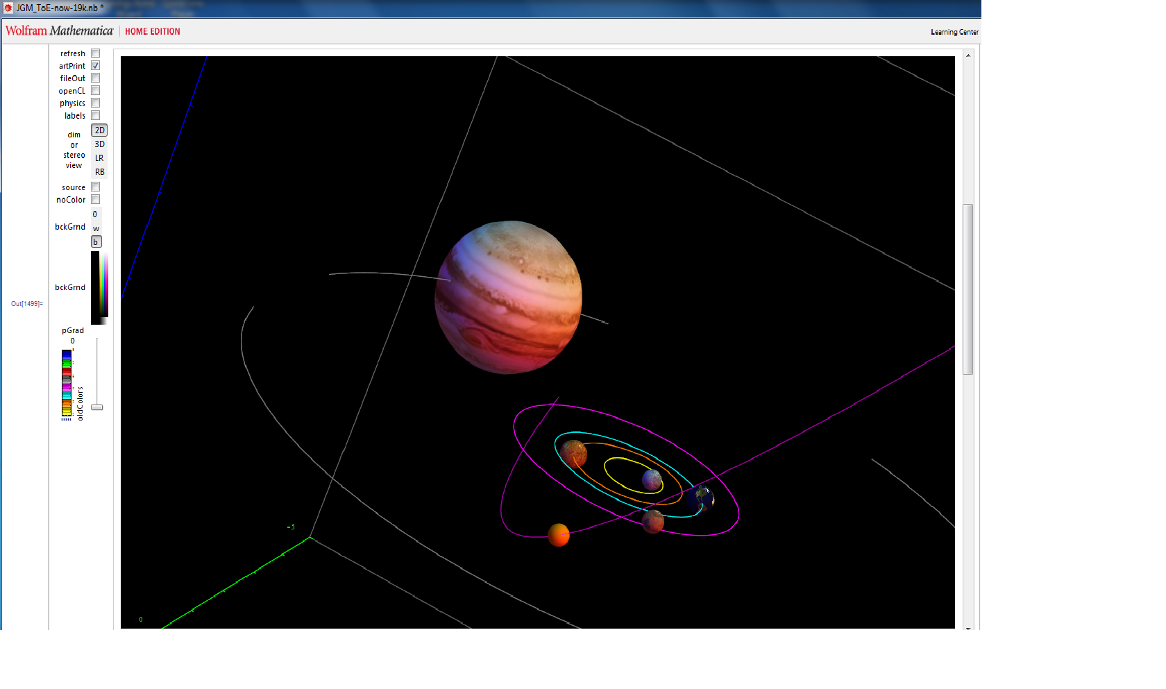
Comet Siding Spring passing by Mars
I’ve been working w/the solar system data plots. Here is my version of the Siding Spring comet orbital path metadata – except with the planets given some scale and surface imagery.
It is created using an interactive CDF viewer available at http://theoryofeverything.org/theToE/visualizations/interactive/ (Selecting the interaction pane for Universal NBody gravitational simulator and selecting the current “Solar System” Epoch.
If you want to create a version yourself, all you need is the free Wolfram CDF player and go to the interactive visualization tool referenced above. Select the NBody Gravitational Universe simulation and select the “Recombination” epoch (the last one on the timeline).
Please note, there are two distance scales (outer planets to start, and quickly switches to inner planets as it gets close to Mars).
The planets are scaled relative to each other in each of these scales, but not relative to the Astronomical Unit distance scale between them.
BTW – The Sun is not shown, since at that planetary scale it is actually bigger than the frame of the animation 🙂
The time scale goes from last year to next year. It changes from linear around this weekend (0s) and goes exponential on the outer orbits.